This tutorial has been forked from awesome classes developed by Adam Wilson here: http://adamwilson.us/RDataScience/

The R Script associated with this page is available here. Download this file and open it (or copy-paste into a new script) with RStudio so you can follow along.

1 RStudio Shortcuts

1.1 Running code

ctrl-R (or command-R) to run current line
Highlight code in script and run ctrl-R (or command-R) to run selection
Buttons:

1.2 Switching windows

ctrl-1: script window
ctrl-2: console window

Try to run today’s script without using your mouse/trackpad

2 Data wrangling

2.1 Useful packages: `dplyr` and `tidyr`

Cheat sheets on website for Data Wrangling

library(dplyr)
library(tidyr)

Remember use install.packages("dplyr") to install a new package.

2.1.1 Example operations from here

2.2 New York City Flights

Data from US Bureau of Transportation Statistics (see ?nycflights13)

library(nycflights13)

Check out the flights object

head(flights)

## # A tibble: 6 × 19
##    year month   day dep_time sched_dep_time
##   <int> <int> <int>    <int>          <int>
## 1  2013     1     1      517            515
## 2  2013     1     1      533            529
## 3  2013     1     1      542            540
## 4  2013     1     1      544            545
## 5  2013     1     1      554            600
## 6  2013     1     1      554            558
## # ... with 14 more variables: dep_delay <dbl>,
## #   arr_time <int>, sched_arr_time <int>,
## #   arr_delay <dbl>, carrier <chr>, flight <int>,
## #   tailnum <chr>, origin <chr>, dest <chr>,
## #   air_time <dbl>, distance <dbl>, hour <dbl>,
## #   minute <dbl>, time_hour <dttm>

2.2.1 Object Structure

Check out data structure with glimpse()

glimpse(flights)

## Observations: 336,776
## Variables: 19
## $ year           <int> 2013, 2013, 2013, 2013...
## $ month          <int> 1, 1, 1, 1, 1, 1, 1, 1...
## $ day            <int> 1, 1, 1, 1, 1, 1, 1, 1...
## $ dep_time       <int> 517, 533, 542, 544, 55...
## $ sched_dep_time <int> 515, 529, 540, 545, 60...
## $ dep_delay      <dbl> 2, 4, 2, -1, -6, -4, -...
## $ arr_time       <int> 830, 850, 923, 1004, 8...
## $ sched_arr_time <int> 819, 830, 850, 1022, 8...
## $ arr_delay      <dbl> 11, 20, 33, -18, -25, ...
## $ carrier        <chr> "UA", "UA", "AA", "B6"...
## $ flight         <int> 1545, 1714, 1141, 725,...
## $ tailnum        <chr> "N14228", "N24211", "N...
## $ origin         <chr> "EWR", "LGA", "JFK", "...
## $ dest           <chr> "IAH", "IAH", "MIA", "...
## $ air_time       <dbl> 227, 227, 160, 183, 11...
## $ distance       <dbl> 1400, 1416, 1089, 1576...
## $ hour           <dbl> 5, 5, 5, 5, 6, 5, 6, 6...
## $ minute         <dbl> 15, 29, 40, 45, 0, 58,...
## $ time_hour      <dttm> 2013-01-01 05:00:00, ...

3 `dplyr` “verbs”

select() and rename(): Extract existing variables
filter() and slice(): Extract existing observations
arrange()
distinct()
mutate() and transmute(): Derive new variables
summarise(): Change the unit of analysis
sample_n() and sample_frac()

3.1 Useful select functions

“-” Select everything but
“:” Select range
contains() Select columns whose name contains a character string
ends_with() Select columns whose name ends with a string
everything() Select every column
matches() Select columns whose name matches a regular expression
num_range() Select columns named x1, x2, x3, x4, x5
one_of() Select columns whose names are in a group of names
starts_with() Select columns whose name starts with a character string

3.1.1 `select()` examples

Select only the year, month, and day columns:

select(flights,year, month, day)

## # A tibble: 336,776 × 3
##     year month   day
##    <int> <int> <int>
## 1   2013     1     1
## 2   2013     1     1
## 3   2013     1     1
## 4   2013     1     1
## 5   2013     1     1
## 6   2013     1     1
## 7   2013     1     1
## 8   2013     1     1
## 9   2013     1     1
## 10  2013     1     1
## # ... with 336,766 more rows

3.1.2 `select()` examples

Select everything except the tailnum:

select(flights,-tailnum)

## # A tibble: 336,776 × 18
##     year month   day dep_time sched_dep_time
##    <int> <int> <int>    <int>          <int>
## 1   2013     1     1      517            515
## 2   2013     1     1      533            529
## 3   2013     1     1      542            540
## 4   2013     1     1      544            545
## 5   2013     1     1      554            600
## 6   2013     1     1      554            558
## 7   2013     1     1      555            600
## 8   2013     1     1      557            600
## 9   2013     1     1      557            600
## 10  2013     1     1      558            600
## # ... with 336,766 more rows, and 13 more
## #   variables: dep_delay <dbl>, arr_time <int>,
## #   sched_arr_time <int>, arr_delay <dbl>,
## #   carrier <chr>, flight <int>, origin <chr>,
## #   dest <chr>, air_time <dbl>, distance <dbl>,
## #   hour <dbl>, minute <dbl>, time_hour <dttm>

Select all columns containing the string "time":

select(flights,contains("time"))

## # A tibble: 336,776 × 6
##    dep_time sched_dep_time arr_time
##       <int>          <int>    <int>
## 1       517            515      830
## 2       533            529      850
## 3       542            540      923
## 4       544            545     1004
## 5       554            600      812
## 6       554            558      740
## 7       555            600      913
## 8       557            600      709
## 9       557            600      838
## 10      558            600      753
## # ... with 336,766 more rows, and 3 more
## #   variables: sched_arr_time <int>,
## #   air_time <dbl>, time_hour <dttm>

You can also rename columns with select()

select(flights,year,carrier,destination=dest)

## # A tibble: 336,776 × 3
##     year carrier destination
##    <int>   <chr>       <chr>
## 1   2013      UA         IAH
## 2   2013      UA         IAH
## 3   2013      AA         MIA
## 4   2013      B6         BQN
## 5   2013      DL         ATL
## 6   2013      UA         ORD
## 7   2013      B6         FLL
## 8   2013      EV         IAD
## 9   2013      B6         MCO
## 10  2013      AA         ORD
## # ... with 336,766 more rows

3.2 `filter()` observations

Filter all flights that departed on on January 1st:

filter(flights, month == 1, day == 1)

## # A tibble: 842 × 19
##     year month   day dep_time sched_dep_time
##    <int> <int> <int>    <int>          <int>
## 1   2013     1     1      517            515
## 2   2013     1     1      533            529
## 3   2013     1     1      542            540
## 4   2013     1     1      544            545
## 5   2013     1     1      554            600
## 6   2013     1     1      554            558
## 7   2013     1     1      555            600
## 8   2013     1     1      557            600
## 9   2013     1     1      557            600
## 10  2013     1     1      558            600
## # ... with 832 more rows, and 14 more variables:
## #   dep_delay <dbl>, arr_time <int>,
## #   sched_arr_time <int>, arr_delay <dbl>,
## #   carrier <chr>, flight <int>, tailnum <chr>,
## #   origin <chr>, dest <chr>, air_time <dbl>,
## #   distance <dbl>, hour <dbl>, minute <dbl>,
## #   time_hour <dttm>

3.3 Base R method

This is equivalent to the more verbose code in base R:

flights[flights$month == 1 & flights$day == 1, ]

## # A tibble: 842 × 19
##     year month   day dep_time sched_dep_time
##    <int> <int> <int>    <int>          <int>
## 1   2013     1     1      517            515
## 2   2013     1     1      533            529
## 3   2013     1     1      542            540
## 4   2013     1     1      544            545
## 5   2013     1     1      554            600
## 6   2013     1     1      554            558
## 7   2013     1     1      555            600
## 8   2013     1     1      557            600
## 9   2013     1     1      557            600
## 10  2013     1     1      558            600
## # ... with 832 more rows, and 14 more variables:
## #   dep_delay <dbl>, arr_time <int>,
## #   sched_arr_time <int>, arr_delay <dbl>,
## #   carrier <chr>, flight <int>, tailnum <chr>,
## #   origin <chr>, dest <chr>, air_time <dbl>,
## #   distance <dbl>, hour <dbl>, minute <dbl>,
## #   time_hour <dttm>

Compare with dplyr method:

filter(flights, month == 1, day == 1)`

Filter the flights data set to keep only evening flights (dep_time after 1600) in June.

filter(flights,dep_time>1600,month==6)

## # A tibble: 10,117 × 19
##     year month   day dep_time sched_dep_time
##    <int> <int> <int>    <int>          <int>
## 1   2013     6     1     1602           1505
## 2   2013     6     1     1602           1605
## 3   2013     6     1     1602           1610
## 4   2013     6     1     1603           1610
## 5   2013     6     1     1603           1545
## 6   2013     6     1     1605           1608
## 7   2013     6     1     1605           1600
## 8   2013     6     1     1605           1614
## 9   2013     6     1     1608           1600
## 10  2013     6     1     1609           1615
## # ... with 10,107 more rows, and 14 more
## #   variables: dep_delay <dbl>, arr_time <int>,
## #   sched_arr_time <int>, arr_delay <dbl>,
## #   carrier <chr>, flight <int>, tailnum <chr>,
## #   origin <chr>, dest <chr>, air_time <dbl>,
## #   distance <dbl>, hour <dbl>, minute <dbl>,
## #   time_hour <dttm>

3.4 Other boolean expressions

filter() is similar to subset() except it handles any number of filtering conditions joined together with &.

You can also use other boolean operators, such as OR (“|”):

filter(flights, month == 1 | month == 2)

## # A tibble: 51,955 × 19
##     year month   day dep_time sched_dep_time
##    <int> <int> <int>    <int>          <int>
## 1   2013     1     1      517            515
## 2   2013     1     1      533            529
## 3   2013     1     1      542            540
## 4   2013     1     1      544            545
## 5   2013     1     1      554            600
## 6   2013     1     1      554            558
## 7   2013     1     1      555            600
## 8   2013     1     1      557            600
## 9   2013     1     1      557            600
## 10  2013     1     1      558            600
## # ... with 51,945 more rows, and 14 more
## #   variables: dep_delay <dbl>, arr_time <int>,
## #   sched_arr_time <int>, arr_delay <dbl>,
## #   carrier <chr>, flight <int>, tailnum <chr>,
## #   origin <chr>, dest <chr>, air_time <dbl>,
## #   distance <dbl>, hour <dbl>, minute <dbl>,
## #   time_hour <dttm>

Filter the flights data set to keep only ‘redeye’ flights where the departure time (dep_time) is “after” the arrival time (arr_time), indicating it arrived the next day:

filter(flights,dep_time>arr_time)

## # A tibble: 10,633 × 19
##     year month   day dep_time sched_dep_time
##    <int> <int> <int>    <int>          <int>
## 1   2013     1     1     1929           1920
## 2   2013     1     1     1939           1840
## 3   2013     1     1     2058           2100
## 4   2013     1     1     2102           2108
## 5   2013     1     1     2108           2057
## 6   2013     1     1     2120           2130
## 7   2013     1     1     2121           2040
## 8   2013     1     1     2128           2135
## 9   2013     1     1     2134           2045
## 10  2013     1     1     2136           2145
## # ... with 10,623 more rows, and 14 more
## #   variables: dep_delay <dbl>, arr_time <int>,
## #   sched_arr_time <int>, arr_delay <dbl>,
## #   carrier <chr>, flight <int>, tailnum <chr>,
## #   origin <chr>, dest <chr>, air_time <dbl>,
## #   distance <dbl>, hour <dbl>, minute <dbl>,
## #   time_hour <dttm>

3.5 Select rows with `slice()`:

slice(flights, 1:10)

## # A tibble: 10 × 19
##     year month   day dep_time sched_dep_time
##    <int> <int> <int>    <int>          <int>
## 1   2013     1     1      517            515
## 2   2013     1     1      533            529
## 3   2013     1     1      542            540
## 4   2013     1     1      544            545
## 5   2013     1     1      554            600
## 6   2013     1     1      554            558
## 7   2013     1     1      555            600
## 8   2013     1     1      557            600
## 9   2013     1     1      557            600
## 10  2013     1     1      558            600
## # ... with 14 more variables: dep_delay <dbl>,
## #   arr_time <int>, sched_arr_time <int>,
## #   arr_delay <dbl>, carrier <chr>, flight <int>,
## #   tailnum <chr>, origin <chr>, dest <chr>,
## #   air_time <dbl>, distance <dbl>, hour <dbl>,
## #   minute <dbl>, time_hour <dttm>

3.6 `arrange()` rows

arrange() is similar to filter() except it reorders instead of filtering.

arrange(flights, year, month, day)

## # A tibble: 336,776 × 19
##     year month   day dep_time sched_dep_time
##    <int> <int> <int>    <int>          <int>
## 1   2013     1     1      517            515
## 2   2013     1     1      533            529
## 3   2013     1     1      542            540
## 4   2013     1     1      544            545
## 5   2013     1     1      554            600
## 6   2013     1     1      554            558
## 7   2013     1     1      555            600
## 8   2013     1     1      557            600
## 9   2013     1     1      557            600
## 10  2013     1     1      558            600
## # ... with 336,766 more rows, and 14 more
## #   variables: dep_delay <dbl>, arr_time <int>,
## #   sched_arr_time <int>, arr_delay <dbl>,
## #   carrier <chr>, flight <int>, tailnum <chr>,
## #   origin <chr>, dest <chr>, air_time <dbl>,
## #   distance <dbl>, hour <dbl>, minute <dbl>,
## #   time_hour <dttm>

Base R method:

flights[order(flights$year, flights$month, flights$day), ]

3.7 Descending order: `desc()`

arrange(flights, desc(arr_delay))

## # A tibble: 336,776 × 19
##     year month   day dep_time sched_dep_time
##    <int> <int> <int>    <int>          <int>
## 1   2013     1     9      641            900
## 2   2013     6    15     1432           1935
## 3   2013     1    10     1121           1635
## 4   2013     9    20     1139           1845
## 5   2013     7    22      845           1600
## 6   2013     4    10     1100           1900
## 7   2013     3    17     2321            810
## 8   2013     7    22     2257            759
## 9   2013    12     5      756           1700
## 10  2013     5     3     1133           2055
## # ... with 336,766 more rows, and 14 more
## #   variables: dep_delay <dbl>, arr_time <int>,
## #   sched_arr_time <int>, arr_delay <dbl>,
## #   carrier <chr>, flight <int>, tailnum <chr>,
## #   origin <chr>, dest <chr>, air_time <dbl>,
## #   distance <dbl>, hour <dbl>, minute <dbl>,
## #   time_hour <dttm>

Base R method:

flights[order(desc(flights$arr_delay)), ]

3.8 Distinct: Find distinct rows

distinct(
  select(flights,carrier)
)

## # A tibble: 16 × 1
##    carrier
##      <chr>
## 1       UA
## 2       AA
## 3       B6
## 4       DL
## 5       EV
## 6       MQ
## 7       US
## 8       WN
## 9       VX
## 10      FL
## 11      AS
## 12      9E
## 13      F9
## 14      HA
## 15      YV
## 16      OO

3.9 Mutate: Derive new variables

Adds columns with calculations based on other columns.

Average air speed (miles/hour):

select(
  mutate(flights,ave_speed=distance/(air_time/60)),
  distance, air_time,ave_speed)

## # A tibble: 336,776 × 3
##    distance air_time ave_speed
##       <dbl>    <dbl>     <dbl>
## 1      1400      227  370.0441
## 2      1416      227  374.2731
## 3      1089      160  408.3750
## 4      1576      183  516.7213
## 5       762      116  394.1379
## 6       719      150  287.6000
## 7      1065      158  404.4304
## 8       229       53  259.2453
## 9       944      140  404.5714
## 10      733      138  318.6957
## # ... with 336,766 more rows

3.10 Chaining Operations

Performing multiple operations sequentially with a pipe character

Group by a variable
Select some columns
Summarize observations
Filter by results

With temporary objects:

a1 <- group_by(flights, year, month, day)
a2 <- select(a1, arr_delay, dep_delay)

## Adding missing grouping variables: `year`, `month`, `day`

a3 <- summarise(a2,
                arr = mean(arr_delay, na.rm = TRUE),
                dep = mean(dep_delay, na.rm = TRUE))
a4 <- filter(a3, arr > 30 | dep > 30)
head(a4)

## Source: local data frame [6 x 5]
## Groups: year, month [3]
## 
##    year month   day      arr      dep
##   <int> <int> <int>    <dbl>    <dbl>
## 1  2013     1    16 34.24736 24.61287
## 2  2013     1    31 32.60285 28.65836
## 3  2013     2    11 36.29009 39.07360
## 4  2013     2    27 31.25249 37.76327
## 5  2013     3     8 85.86216 83.53692
## 6  2013     3    18 41.29189 30.11796

If you don’t want to save the intermediate results: wrap the function calls inside each other:

filter(
  summarise(
    select(
      group_by(flights, year, month, day),
      arr_delay, dep_delay
    ),
    arr = mean(arr_delay, na.rm = TRUE),
    dep = mean(dep_delay, na.rm = TRUE)
  ),
  arr > 30 | dep > 30
)

## Adding missing grouping variables: `year`, `month`, `day`

## Source: local data frame [49 x 5]
## Groups: year, month [11]
## 
##     year month   day      arr      dep
##    <int> <int> <int>    <dbl>    <dbl>
## 1   2013     1    16 34.24736 24.61287
## 2   2013     1    31 32.60285 28.65836
## 3   2013     2    11 36.29009 39.07360
## 4   2013     2    27 31.25249 37.76327
## 5   2013     3     8 85.86216 83.53692
## 6   2013     3    18 41.29189 30.11796
## 7   2013     4    10 38.41231 33.02368
## 8   2013     4    12 36.04814 34.83843
## 9   2013     4    18 36.02848 34.91536
## 10  2013     4    19 47.91170 46.12783
## # ... with 39 more rows

Arguments are distant from function -> difficult to read!

3.11 Chaining Operations

%>% allows you to pipe together various commands

x %>% f(y) turns into f(x, y)

So you can use it to rewrite multiple operations that you can read left-to-right, top-to-bottom:

flights %>%
  group_by(year, month, day) %>%
  select(arr_delay, dep_delay) %>%
  summarise(
    arr = mean(arr_delay, na.rm = TRUE),
    dep = mean(dep_delay, na.rm = TRUE)
  ) %>%
  filter(arr > 30 | dep > 30)

## Adding missing grouping variables: `year`, `month`, `day`

## Source: local data frame [49 x 5]
## Groups: year, month [11]
## 
##     year month   day      arr      dep
##    <int> <int> <int>    <dbl>    <dbl>
## 1   2013     1    16 34.24736 24.61287
## 2   2013     1    31 32.60285 28.65836
## 3   2013     2    11 36.29009 39.07360
## 4   2013     2    27 31.25249 37.76327
## 5   2013     3     8 85.86216 83.53692
## 6   2013     3    18 41.29189 30.11796
## 7   2013     4    10 38.41231 33.02368
## 8   2013     4    12 36.04814 34.83843
## 9   2013     4    18 36.02848 34.91536
## 10  2013     4    19 47.91170 46.12783
## # ... with 39 more rows

3.12 Analyze by group with `group_by()`

Perform operations by group: mean departure delay by airport (origin)

flights %>%
  group_by(origin) %>%
  summarise(meanDelay = mean(dep_delay,na.rm=T))

## # A tibble: 3 × 2
##   origin meanDelay
##    <chr>     <dbl>
## 1    EWR  15.10795
## 2    JFK  12.11216
## 3    LGA  10.34688

Perform operations by group: mean and sd departure delay by airline (carrier)

flights %>% 
  group_by(carrier) %>%  
  summarise(meanDelay = mean(dep_delay,na.rm=T),
            sdDelay =   sd(dep_delay,na.rm=T))

## # A tibble: 16 × 3
##    carrier meanDelay  sdDelay
##      <chr>     <dbl>    <dbl>
## 1       9E 16.725769 45.90604
## 2       AA  8.586016 37.35486
## 3       AS  5.804775 31.36303
## 4       B6 13.022522 38.50337
## 5       DL  9.264505 39.73505
## 6       EV 19.955390 46.55235
## 7       F9 20.215543 58.36265
## 8       FL 18.726075 52.66160
## 9       HA  4.900585 74.10990
## 10      MQ 10.552041 39.18457
## 11      OO 12.586207 43.06599
## 12      UA 12.106073 35.71660
## 13      US  3.782418 28.05633
## 14      VX 12.869421 44.81510
## 15      WN 17.711744 43.34435
## 16      YV 18.996330 49.17227

Flights from which origin airport go the farthest (on average)? Hint: Group by airport (origin) then calculate the maximum flight distance (distance).

flights %>% 
  group_by(origin) %>%  
  summarise(meanDist = mean(distance,na.rm=T))

## # A tibble: 3 × 2
##   origin  meanDist
##    <chr>     <dbl>
## 1    EWR 1056.7428
## 2    JFK 1266.2491
## 3    LGA  779.8357

Which destination airport (dest) is the farthest (distance) from NYC?

flights %>% 
  arrange(desc(distance)) %>% 
  select(dest,distance) %>% 
  slice(1)

## # A tibble: 1 × 2
##    dest distance
##   <chr>    <dbl>
## 1   HNL     4983

Which airport is that?

4 Combining data sets

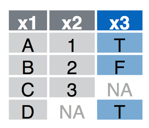
4.1 `dplyr` join methods

Drawing

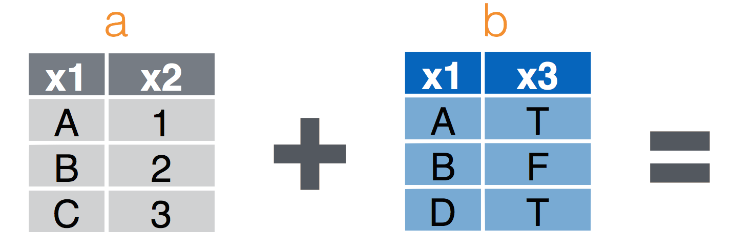
left_join(a, b, by = "x1") Join matching rows from b to a.
right_join(a, b, by = "x1") Join matching rows from a to b.
inner_join(a, b, by = "x1") Retain only rows in both sets.
full_join(a, b, by = "x1") Join data. Retain all values, all rows.

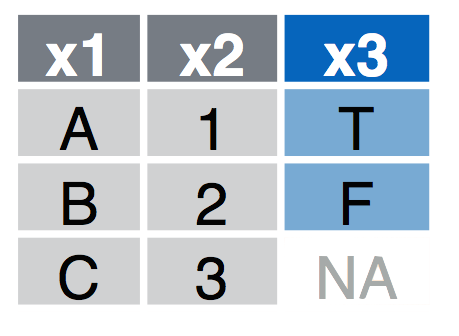
4.1.1 Left Join

left_join(a, b, by = "x1") Join matching rows from b to a.

Drawing Drawing

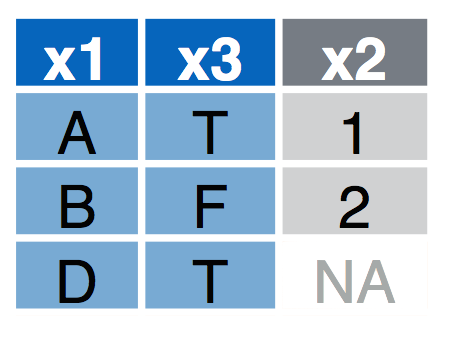
4.1.2 Right Join

right_join(a, b, by = "x1") Join matching rows from a to b.

Drawing Drawing

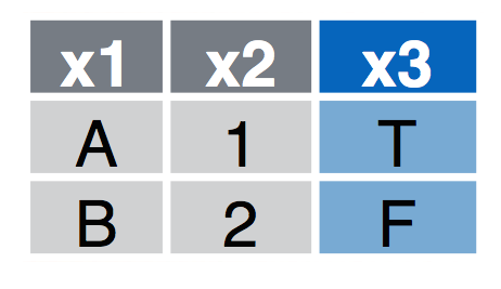
4.1.3 Inner Join

inner_join(a, b, by = "x1") Retain only rows in both sets.

Drawing Drawing

4.1.4 Full Join

full_join(a, b, by = "x1") Join data. Retain all values, all rows.

Drawing Drawing

flights%>%
  select(-year,-month,-day,-hour,-minute,-dep_time,-dep_delay)%>%
  glimpse()

## Observations: 336,776
## Variables: 12
## $ sched_dep_time <int> 515, 529, 540, 545, 60...
## $ arr_time       <int> 830, 850, 923, 1004, 8...
## $ sched_arr_time <int> 819, 830, 850, 1022, 8...
## $ arr_delay      <dbl> 11, 20, 33, -18, -25, ...
## $ carrier        <chr> "UA", "UA", "AA", "B6"...
## $ flight         <int> 1545, 1714, 1141, 725,...
## $ tailnum        <chr> "N14228", "N24211", "N...
## $ origin         <chr> "EWR", "LGA", "JFK", "...
## $ dest           <chr> "IAH", "IAH", "MIA", "...
## $ air_time       <dbl> 227, 227, 160, 183, 11...
## $ distance       <dbl> 1400, 1416, 1089, 1576...
## $ time_hour      <dttm> 2013-01-01 05:00:00, ...

Let’s look at the airports data table (?airports for documentation):

glimpse(airports)

## Observations: 1,396
## Variables: 7
## $ faa  <chr> "04G", "06A", "06C", "06N", "09J...
## $ name <chr> "Lansdowne Airport", "Moton Fiel...
## $ lat  <dbl> 41.13047, 32.46057, 41.98934, 41...
## $ lon  <dbl> -80.61958, -85.68003, -88.10124,...
## $ alt  <int> 1044, 264, 801, 523, 11, 1593, 7...
## $ tz   <dbl> -5, -5, -6, -5, -4, -4, -5, -5, ...
## $ dst  <chr> "A", "A", "A", "A", "A", "A", "A...

What is the name of the destination airport farthest from the NYC airports? Hints:

Use a join to connect the flights dataset and airports dataset.
Figure out which column connects the two tables.
You may need to rename the column names before joining.

select(airports,
       dest=faa,
       destName=name)%>%
  right_join(flights)%>% 
  arrange(desc(distance)) %>% 
  slice(1) %>% 
  select(destName)

## Joining, by = "dest"

## # A tibble: 1 × 1
##        destName
##           <chr>
## 1 Honolulu Intl

4.2 Plot the `flights` data

The section below shows some ‘advanced’ coding to extract the geographic locations for all flights and plotting. This is just meant as an example to illustrate how one might use these functions to perform a mini-analysis that results in a map.

4.2.1 Join destination airports

library(geosphere)
library(maps)
library(ggplot2)
library(sp)
library(rgeos)

## rgeos version: 0.3-21, (SVN revision 540)
##  GEOS runtime version: 3.4.2-CAPI-1.8.2 r3921 
##  Linking to sp version: 1.2-3 
##  Polygon checking: TRUE

data=
  select(airports,
         dest=faa,
         destName=name,
         destLat=lat,
         destLon=lon)%>%
  right_join(flights)%>%
  group_by(dest,
           destLon,
           destLat,
           distance)%>%
  summarise(count=n())%>%
  ungroup()%>%
  select(destLon,
         destLat,
         count,
         distance)%>%
  mutate(id=row_number())%>%
  na.omit()

## Joining, by = "dest"

NYCll=airports%>%filter(faa=="JFK")%>%select(lon,lat)  # get NYC coordinates

# calculate great circle routes
rts <- gcIntermediate(as.matrix(NYCll),
                      as.matrix(select(data,destLon,destLat)),
                      1000,
                      addStartEnd=TRUE,
                      sp=TRUE)

## NOTE: rgdal::checkCRSArgs: no proj_defs.dat in PROJ.4 shared files

rts.ff <- fortify(
  as(rts,"SpatialLinesDataFrame")) # convert into something ggplot can plot

## join with count of flights
rts.ff$id=as.integer(rts.ff$id)
gcircles <- left_join(rts.ff,
                      data,
                      by="id") # join attributes, we keep them all, just in case

Now build a basemap using data in the maps package.

base = ggplot()
worldmap <- map_data("world",
                     ylim = c(10, 70),
                     xlim = c(-160, -80))
wrld <- c(geom_polygon(
  aes(long, lat, group = group),
  size = 0.1,
  colour = "grey",
  fill = "grey",
  alpha = 1,
  data = worldmap
))

Now draw the map using ggplot

base + wrld +
  geom_path(
    data = gcircles,
    aes(
      long,
      lat,
      col = count,
      group = group,
      order = as.factor(distance)
    ),
    alpha = 0.5,
    lineend = "round",
    lwd = 1
  ) +
  coord_equal() +
  scale_colour_gradientn(colours = c("blue", "orange", "red"),
                         guide = "colourbar") +
  theme(panel.background = element_rect(fill = 'white', colour = 'white')) +
  labs(y = "Latitude", x = "Longitude",
       title = "Count of Flights from New York in 2013")

## Warning: Ignoring unknown aesthetics: order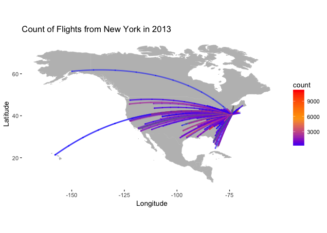

4.3 Colophon

This exercise based on code from here.

Data Wrangling

1 RStudio Shortcuts

1.1 Running code

1.2 Switching windows

2 Data wrangling

2.1 Useful packages: dplyr and tidyr

2.1.1 Example operations from here

2.2 New York City Flights

2.2.1 Object Structure

3 dplyr “verbs”

3.1 Useful select functions

3.1.1 select() examples

3.1.2 select() examples

3.2 filter() observations

3.3 Base R method

3.4 Other boolean expressions

3.5 Select rows with slice():

3.6 arrange() rows

3.7 Descending order: desc()

3.8 Distinct: Find distinct rows

3.9 Mutate: Derive new variables

3.10 Chaining Operations

3.11 Chaining Operations

3.12 Analyze by group with group_by()

4 Combining data sets

4.1 dplyr join methods

4.1.1 Left Join

4.1.2 Right Join

4.1.3 Inner Join

4.1.4 Full Join

4.2 Plot the flights data

4.2.1 Join destination airports

4.3 Colophon

2.1 Useful packages: `dplyr` and `tidyr`

3 `dplyr` “verbs”

3.1.1 `select()` examples

3.1.2 `select()` examples

3.2 `filter()` observations

3.5 Select rows with `slice()`:

3.6 `arrange()` rows

3.7 Descending order: `desc()`

3.12 Analyze by group with `group_by()`

4.1 `dplyr` join methods

4.2 Plot the `flights` data