Introduction to Integral Projection Models
Cory Merow
10/5/2017
This tutorial gives a practical overview of building stage-structured (e.g. size, age) population models use integral projection models.
Download the PDF of the presentation
The R Script associated with this page is available
1 Introductory IPM exercises
Here, we introduce a simple IPM for a the long-lived alpine perennial plant Dracocephalum austriacum. The analyses minimize the complexity of the R code in order to make the model transparent. We calculate basic population statistics, including population growth rate, sensitivity, elasticity, and passage times throughout to check the plausibility of the model.
The document is organized as follows
- plots for data exploration
- parameter estimation for regressions
- build vital rate functions
- make a kernel
- basic analyses
2 Data exploration
To read in the data you’ll have to set your own file path here.
d=read.csv('21_assets/Exercises/Intro_to_IPMs_Exercises_Data.csv')You’ll notice that adults are stored at the beginning of the data set with values for size (measured in 2001) and sizeNext (measured in 2002). the number of seeds and flowering status were measured in 2001.
head(d)New recruits are stored at the end and were only observed in the second survey (2002). Hence their size value is NA and sizeNext value is an integer.
tail(d) # make some plots - figure 1
par(mfrow=c(2,2),mar=c(4,4,2,1))
plot(d$size,jitter(d$surv),main='Survival') # jittered to see easier
plot(d$size,d$sizeNext,main='Growth/Shrinkage/Stasis')
plot(d$size,d$fec.seed,main='Seeds') # jittered to see easier
hist(d$sizeNext[is.na(d$size)],main='Size of Recruits')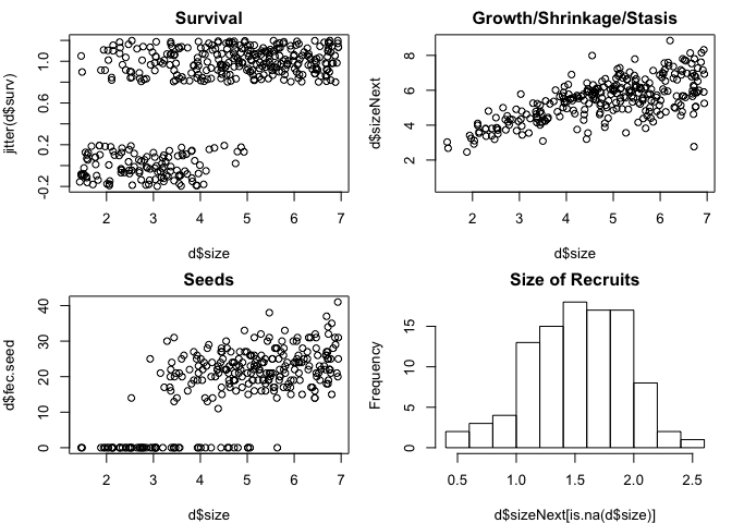
Note that we use NAs for missing or non-applicable data rather than 0 or some other indicator because this causes them to be automatically excluded from r’s regression functions.
The model we’ll build takes the general form (note that equations may not render in all browsers)
$ n[z’,t+1]= $
where z’ is size at time t+1 and z is size at time t. P is the growth/survival kernel and F is the fecundity kernel. these will be decomposed further as:
$ P[z’,z]=growth[z’,z] * survival[z] $
$ F[z’,z]=floweringProbability[z] * seedsPerIndividual[z] * establishmentProbability * recruitSize[z’] $
We’ll begin building the regressions for each of these vital rates in the next section.
3 Regressions for vital rate functions
# 0. set up parameter list for regressions
    # this sets up a list of the model parameters. these parameters will be estimated and recorded below.
params=data.frame(
    surv.int=NA,
    surv.slope=NA,
    growth.int=NA,
    growth.slope=NA,
    growth.sd=NA,
    seed.int=NA,
    seed.slope=NA,
    recruit.size.mean=NA,
    recruit.size.sd=NA,
    establishment.prob=NA
)

# 1. survival regression
surv.reg=glm(surv~size,data=d,family=binomial())
summary(surv.reg)
##
## Call:
## glm(formula = surv ~ size, family = binomial(), data = d)
##
## Deviance Residuals:
## Min 1Q Median 3Q Max
## -2.2275 -0.5815 0.2491 0.5597 2.0972
##
## Coefficients:
## Estimate Std. Error z value Pr(>|z|)
## (Intercept) -3.9646 0.4760 -8.329 <2e-16 ***
## size 1.2897 0.1338 9.642 <2e-16 ***
## ---
## Signif. codes: 0 '***' 0.001 '**' 0.01 '*' 0.05 '.' 0.1 ' ' 1
##
## (Dispersion parameter for binomial family taken to be 1)
##
## Null deviance: 488.69 on 399 degrees of freedom
## Residual deviance: 315.82 on 398 degrees of freedom
## (100 observations deleted due to missingness)
## AIC: 319.82
##
## Number of Fisher Scoring iterations: 5params$surv.int=coefficients(surv.reg)[1]
params$surv.slope=coefficients(surv.reg)[2]
# 2. growth regression
growth.reg=lm(sizeNext~size,data=d)
summary(growth.reg)##
## Call:
## lm(formula = sizeNext ~ size, data = d)
##
## Residuals:
## Min 1Q Median 3Q Max
## -3.8037 -0.5434 0.0932 0.5741 2.6732
##
## Coefficients:
## Estimate Std. Error t value Pr(>|t|)
## (Intercept) 2.68135 0.19580 13.69 <2e-16 ***
## size 0.57922 0.03902 14.84 <2e-16 ***
## ---
## Signif. codes: 0 '***' 0.001 '**' 0.01 '*' 0.05 '.' 0.1 ' ' 1
##
## Residual standard error: 0.8866 on 278 degrees of freedom
## (220 observations deleted due to missingness)
## Multiple R-squared: 0.4421, Adjusted R-squared: 0.4401
## F-statistic: 220.3 on 1 and 278 DF, p-value: < 2.2e-16params$growth.int=coefficients(growth.reg)[1]
params$growth.slope=coefficients(growth.reg)[2]
params$growth.sd=sd(resid(growth.reg))# 3. seeds regression
# note that we are just pooling all individuals into this regression regardless of whether they flowered or not. a later exercise will be to explicitly model flowering probability. i.e. for the moment we're taking floweringProbability[z]=1.
seed.reg=glm(fec.seed~size,data=d,family=poisson())
summary(seed.reg)##
## Call:
## glm(formula = fec.seed ~ size, family = poisson(), data = d)
##
## Deviance Residuals:
## Min 1Q Median 3Q Max
## -6.5338 -1.8830 0.0529 1.5375 4.9690
##
## Coefficients:
## Estimate Std. Error z value Pr(>|z|)
## (Intercept) 1.33234 0.06370 20.92 <2e-16 ***
## size 0.30647 0.01164 26.34 <2e-16 ***
## ---
## Signif. codes: 0 '***' 0.001 '**' 0.01 '*' 0.05 '.' 0.1 ' ' 1
##
## (Dispersion parameter for poisson family taken to be 1)
##
## Null deviance: 2598.3 on 279 degrees of freedom
## Residual deviance: 1840.1 on 278 degrees of freedom
## (220 observations deleted due to missingness)
## AIC: 2942.2
##
## Number of Fisher Scoring iterations: 5params$seed.int=coefficients(seed.reg)[1]
params$seed.slope=coefficients(seed.reg)[2]
# 4. size distribution of recruits
# in the dataframe, recruits are those individuals who have a value for sizeNext but not for size
params$recruit.size.mean=mean(d$sizeNext[is.na(d$size)])
params$recruit.size.sd=sd(d$sizeNext[is.na(d$size)])
# 5. establishment probability
# these data represent a single year's worth of data, hence establishment probability can be estimated by dividing the number of observed recruits by the number of seeds. hence the growth/survival measurements were taken in year t which the recruit sizes were measured in year t+1.
params$establishment.prob=sum(is.na(d$size))/sum(d$fec.seed,na.rm=TRUE)
# 6. plot the models over the data - figure 2
par(mfrow=c(2,2),mar=c(4,4,2,1))
xx=seq(0,8,by=.01)
plot(d$size,d$sizeNext,main='Growth/Shrinkage/Stasis')
lines(xx,predict(growth.reg,data.frame(size=xx)),col='red',lwd=3)
plot(d$size,jitter(d$surv),main='Survival') # jittered to see easier
lines(xx,predict(surv.reg,data.frame(size=xx),type='response'), col='red',lwd=3)
plot(d$size,d$fec.seed,main='Seeds') # jittered to see easier
lines(xx,predict(seed.reg,data.frame(size=xx),type='response'), col='red',lwd=3)
hist(d$sizeNext[is.na(d$size)],main='Size of Recruits',freq=FALSE)
lines(xx,dnorm(xx,params$recruit.size.mean,params$recruit.size.sd), col='red',lwd=3)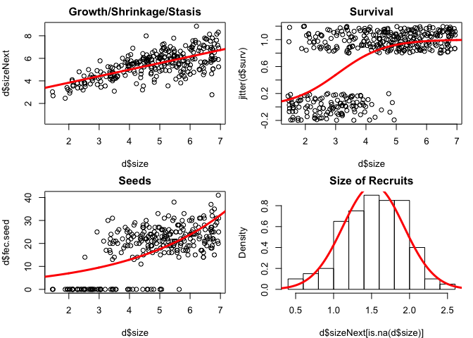
4 Build vital rate functions
Each of the functions below represents one or more of the vital rates. these functions are used to build the IPM and use output (the coefficients) from the regressions developed above.
These functions represent the modeler’s decision about how to decompose the life cycle. in this very simple example, we model (1) survival, (2) growth, (3) seed number, (4) the seedling size distribution and (5) the establishment probability. these last three functions are combined in the model for fecundity below. in practice, we’d need to decide what regressions to build in part B in advance, but it’s easier to digest this section after you’ve seen the regressions above, so fortunately we built all the right regressions already. in practice, sections B and C are iterative one might inform one another.
## vital rate functions

# 1. probability of surviving
# this is a logistic funcion
s.x=function(x,params) {
    u=exp(params$surv.int+params$surv.slope*x)
    return(u/(1+u))
}

# 2. growth function
# this is a normal distribution
g.yx=function(xp,x,params) {
    dnorm(xp,mean=params$growth.int+params$growth.slope*x,sd=params$growth.sd)
}

# 3. reproduction function
# this is a constant times a normal distribution times an exponential function
f.yx=function(xp,x,params) {
    params$establishment.prob*
    dnorm(xp,mean=params$recruit.size.mean,sd=params$recruit.size.sd)*
    exp(params$seed.int+params$seed.slope*x)
}
5 Make a kernel
In this section, we combine the vital rate functions to build the discretized IPM kernel, which we’ll call the IPM matrix (e.g. shown in Fig. 2c in the main text). To integrate, we begin by defining the boundary points (b; the edges of the cells defining the matrix), mesh points (y; the centers of the cells defining the matrix and the points at which the matrix is evaluated for the midpoint rule of numerical integration), and step size (h; the widths of the cells). The integration limits (min.size and max.size) span the range of sizes observed in the data set, and then some.
# 1. boundary points b, mesh points y and step size h
    # integration limits - these limits span the range of sizes observed in the data set, and then some.
min.size=.9*min(c(d$size,d$sizeNext),na.rm=T)
max.size=1.1*max(c(d$size,d$sizeNext),na.rm=T)
    # number of cells in the discretized kernel
n=100
    # boundary points (the edges of the cells defining the kernel)
b=min.size+c(0:n)*(max.size-min.size)/n
# mesh points (midpoints of the cells)
y=0.5*(b[1:n]+b[2:(n+1)])
# width of the cells
h=y[2]-y[1]
Next, we make the IPM matrices. The function outer() evaluates the matrix at all pairwise combinations of the two vectors y and y and returns matrices representing the kernel components for growth and fecundity, respectively. For the numerical integration, we’re using the midpoint rule (the simplest option) to estimate the area under a curve. The midpoint rule assumes a rectangular approximation. The heights of the rectangles are given by the outer function and the width of the rectangles is h.
# 2. make component kernels
par(mfrow=c(2,3))

G=h*outer(y,y,g.yx,params=params)   # growth kernel
image(y,y,t(G),main='growth kernel')        # plot it

S=s.x(y,params=params)                          # survival
plot(y,S,type='l',main='survival')  # plot it

P=G                                                                 # placeholder;redefine P on the next line
for(i in 1:n) P[,i]=G[,i]*S[i]          # growth/survival kernel
image(y,y,t(P),main='survival/growth kernel')   # plot it
abline(0,1,lwd=3)                                       # plot 1:1, which represents stasis

F=h*outer(y,y,f.yx,params=params)   # reproduction kernel
image(y,y,t(F),main='fecundity kernel') # plot it

K=P+F                                                           # full kernel
image(y,y,t(K),main='full kernel')          # plot it

# sometimes it's hard to see both the fecundity part of the kernel swamps the growth/survival part, so here's a plotting trick to level out the kernel
image(y,y,t(K)^.3,main='full kernel^0.3')           # plot it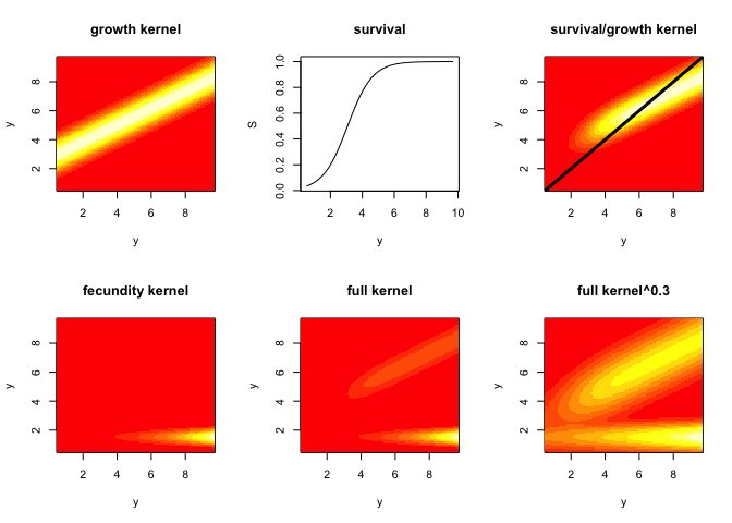
So what did the outer function just do to make the kernel? the way we’ve used it, it takes all pairwise combinations of the the first argument (y) with the second (also y), and does some operation to those combinations. Here are a few examples:
tmp1=outer(y,y,'+')
image(y,y,t(tmp1))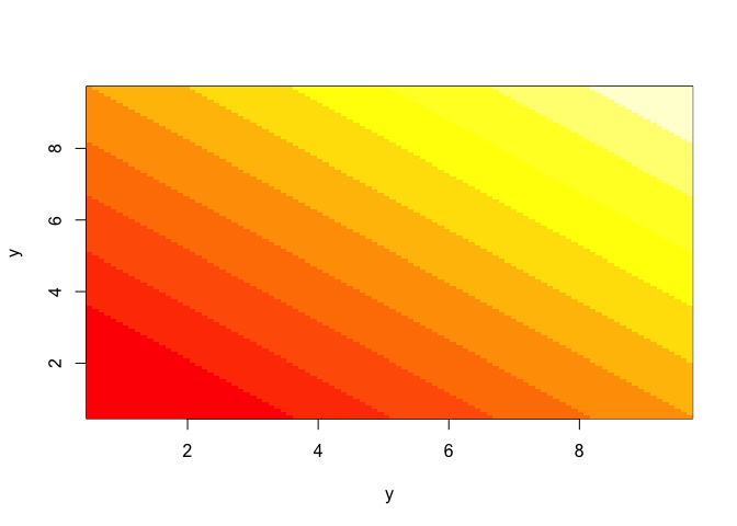
tmp2=outer(y,y,'*')
image(y,y,t(tmp2))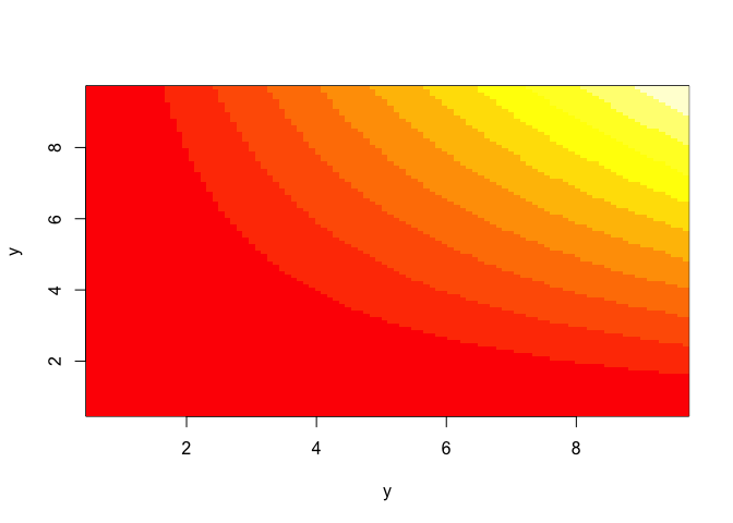
tmp3=outer(y,exp(y),'+')
image(y,exp(y),t(tmp3))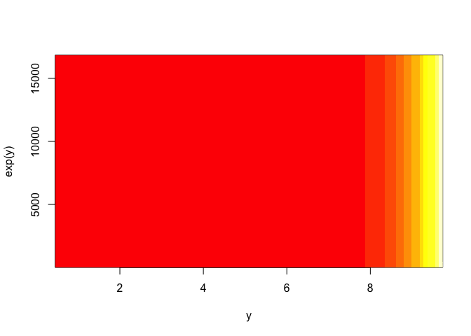 In the IPM case, the operation that we want is not a simple ‘+’ or ’*‘, but the slightly more complicated growth function, given in the third argument (g.yx). to use the growth function, we need to specify the regression coefficients, so the fourth argument supplies the list ’params’ that we defined above, which aer passed to g.yx.
6 Population Summaries
Analyses usually begin with obtaining the eigenvalues (λ) and eigenvectors (v-left; w-right) of the matrix. These are useful for understanding the asymptotic dynamics. The dominant eigenvalue gives the asymptotic population growth rate (lam). The right eigenvector gives the stable stage distribution and the left eigenvector gives the reproductive value, when normalized.
# 1. get lamda,v,w
(lam=Re(eigen(K)$values[1])) # should be 1.013391
## [1] 1.013391w.eigen=Re(eigen(K)$vectors[,1])
stable.dist=w.eigen/sum(w.eigen)
v.eigen=Re(eigen(t(K))$vectors[,1])
repro.val=v.eigen/v.eigen[1]
# The eigen-things can be combined to obtain the sensitivity and elasticity matrices.
# 2. compute elasticity and sensitivity matrices
v.dot.w=sum(stable.dist*repro.val)*h
sens=outer(repro.val,stable.dist)/v.dot.w
elas=matrix(as.vector(sens)*as.vector(K)/lam,nrow=n)
# 3. plot results
par(mfrow=c(2,3))
image(y,y,t(K), xlab="Size (t)",ylab="Size (t+1)",col=topo.colors(100), main="Kernel")
contour(y,y,t(K), add = TRUE, drawlabels = TRUE)
plot(y,stable.dist,xlab="Size",type="l",main="Stable size distribution")
plot(y,repro.val,xlab="Size",type="l",main="Reproductive values")
image(y,y,t(elas),xlab="Size (t)",ylab="Size (t+1)",main="Elasticity")
image(y,y,t(sens),xlab="Size (t)",ylab="Size (t+1)", main="Sensitivity")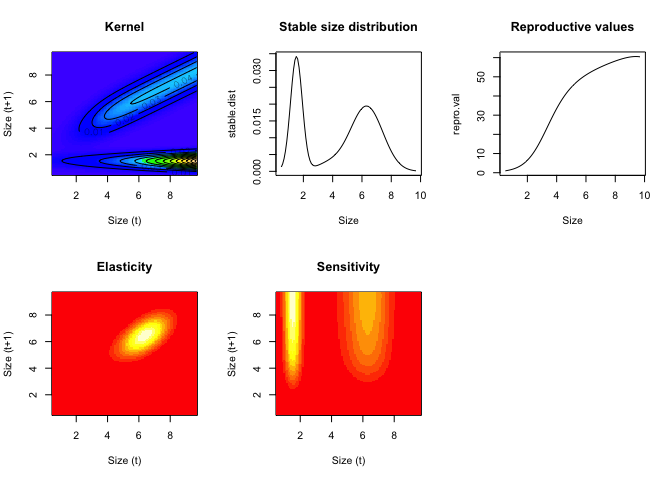
7 Links to Species’ Ranges
Thus far we have fit vital rate models (growth, survival, fecundity) assuming that all individuals experience the same environmental conditions. These models use environmental coavariates in the vital rate regressions to characterize environmental conditions. Using GIS information on how environmental conditions vary across a landscape allows you to predict the vital rates across the landscape and build population models there.
Linked below are some more advanced exercises that reproduce a simplified version of the analysis from my paper on garlic mustard invasion in the northeast US.