The R Script associated with this page is available here. Download this file and open it (or copy-paste into a new script) with RStudio so you can follow along.

This tutorial has been forked from awesome classes developed by Adam Wilson here

1 Setup

library(dplyr)
library(tidyr)
library(sp)
library(ggplot2)
library(rgeos)
library(maptools)
library(rgdal)
library(raster)
library(rasterVis)  #visualization library for raster

2 Point data

2.1 Generate some random data

coords = data.frame(
  x=rnorm(100),
  y=rnorm(100)
)
str(coords)

## 'data.frame':    100 obs. of  2 variables:
##  $ x: num  1.996 0.103 0.239 0.83 -0.323 ...
##  $ y: num  -0.421 -1.103 0.222 -0.753 -0.833 ...

plot(coords)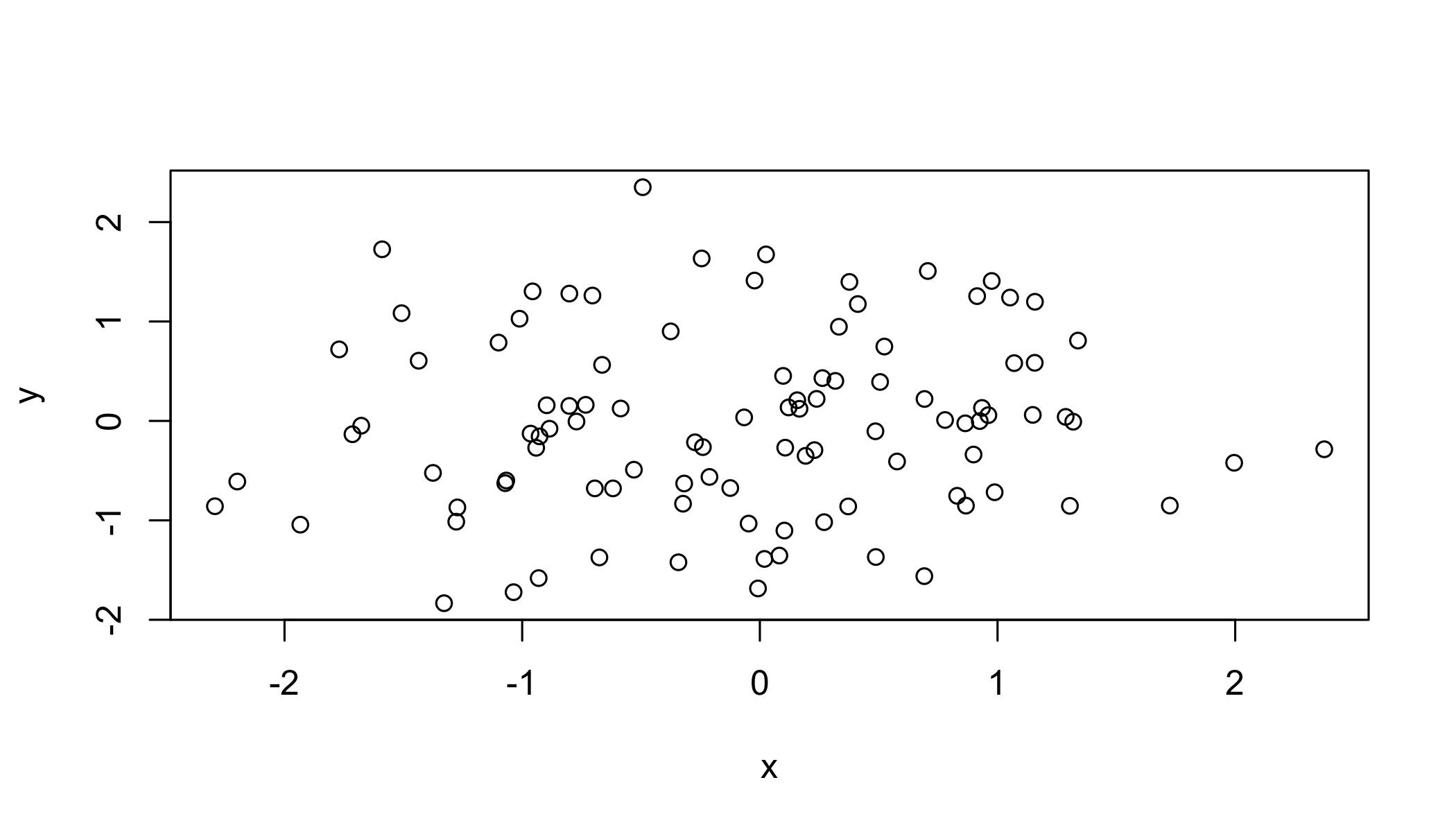

2.2 Convert to `SpatialPoints`

Many tools are designed in R to work specifically with spatial point data, so we need a special object of class SpatialPoints. The important thing is that it has a slot to store coordinates.

sp = SpatialPoints(coords)
str(sp)

## Formal class 'SpatialPoints' [package "sp"] with 3 slots
##   ..@ coords     : num [1:100, 1:2] 1.996 0.103 0.239 0.83 -0.323 ...
##   .. ..- attr(*, "dimnames")=List of 2
##   .. .. ..$ : NULL
##   .. .. ..$ : chr [1:2] "x" "y"
##   ..@ bbox       : num [1:2, 1:2] -2.29 -1.83 2.37 2.35
##   .. ..- attr(*, "dimnames")=List of 2
##   .. .. ..$ : chr [1:2] "x" "y"
##   .. .. ..$ : chr [1:2] "min" "max"
##   ..@ proj4string:Formal class 'CRS' [package "sp"] with 1 slot
##   .. .. ..@ projargs: chr NA

2.3 Create a `SpatialPointsDataFrame`

First generate a dataframe (analagous to the attribute table in a shapefile)

data=data.frame(ID=1:100,group=letters[1:20])
head(data)

##   ID group
## 1  1     a
## 2  2     b
## 3  3     c
## 4  4     d
## 5  5     e
## 6  6     f

Combine the coordinates with the data

spdf = SpatialPointsDataFrame(coords, data)
spdf = SpatialPointsDataFrame(sp, data)

str(spdf)

## Formal class 'SpatialPointsDataFrame' [package "sp"] with 5 slots
##   ..@ data       :'data.frame':  100 obs. of  2 variables:
##   .. ..$ ID   : int [1:100] 1 2 3 4 5 6 7 8 9 10 ...
##   .. ..$ group: Factor w/ 20 levels "a","b","c","d",..: 1 2 3 4 5 6 7 8 9 10 ...
##   ..@ coords.nrs : num(0) 
##   ..@ coords     : num [1:100, 1:2] 1.996 0.103 0.239 0.83 -0.323 ...
##   .. ..- attr(*, "dimnames")=List of 2
##   .. .. ..$ : NULL
##   .. .. ..$ : chr [1:2] "x" "y"
##   ..@ bbox       : num [1:2, 1:2] -2.29 -1.83 2.37 2.35
##   .. ..- attr(*, "dimnames")=List of 2
##   .. .. ..$ : chr [1:2] "x" "y"
##   .. .. ..$ : chr [1:2] "min" "max"
##   ..@ proj4string:Formal class 'CRS' [package "sp"] with 1 slot
##   .. .. ..@ projargs: chr NA

Note the use of slots designated with a @. See ?slot for more.

2.4 Promote a data frame with `coordinates()` to a `SpatialPoints` object

coordinates(data) = cbind(coords$x, coords$y)

str(spdf)

## Formal class 'SpatialPointsDataFrame' [package "sp"] with 5 slots
##   ..@ data       :'data.frame':  100 obs. of  2 variables:
##   .. ..$ ID   : int [1:100] 1 2 3 4 5 6 7 8 9 10 ...
##   .. ..$ group: Factor w/ 20 levels "a","b","c","d",..: 1 2 3 4 5 6 7 8 9 10 ...
##   ..@ coords.nrs : num(0) 
##   ..@ coords     : num [1:100, 1:2] 1.996 0.103 0.239 0.83 -0.323 ...
##   .. ..- attr(*, "dimnames")=List of 2
##   .. .. ..$ : NULL
##   .. .. ..$ : chr [1:2] "x" "y"
##   ..@ bbox       : num [1:2, 1:2] -2.29 -1.83 2.37 2.35
##   .. ..- attr(*, "dimnames")=List of 2
##   .. .. ..$ : chr [1:2] "x" "y"
##   .. .. ..$ : chr [1:2] "min" "max"
##   ..@ proj4string:Formal class 'CRS' [package "sp"] with 1 slot
##   .. .. ..@ projargs: chr NA

2.5 Subset data

subset(spdf, group=="a")

## class       : SpatialPointsDataFrame 
## features    : 5 
## extent      : -1.589283, 1.995578, -0.4209843, 1.726206  (xmin, xmax, ymin, ymax)
## coord. ref. : NA 
## variables   : 2
## names       : ID, group 
## min values  :  1,     a 
## max values  : 81,     a

Or using []

spdf[spdf$group=="a",]

## class       : SpatialPointsDataFrame 
## features    : 5 
## extent      : -1.589283, 1.995578, -0.4209843, 1.726206  (xmin, xmax, ymin, ymax)
## coord. ref. : NA 
## variables   : 2
## names       : ID, group 
## min values  :  1,     a 
## max values  : 81,     a

2.5 Your turn

Convert the following data.frame into a SpatialPointsDataFrame using the coordinates() method and then plot the points with plot().

df=data.frame(
  lat=c(12,15,17,12),
  lon=c(-35,-35,-32,-32),
  id=c(1,2,3,4))

lat	lon	id
12	-35	1
15	-35	2
17	-32	3
12	-32	4

coordinates(df)=c("lon","lat")
plot(df)

2.6 Examine topsoil quality in the Meuse river data set

## Load the data
data(meuse)
str(meuse)

## 'data.frame':    155 obs. of  14 variables:
##  $ x      : num  181072 181025 181165 181298 181307 ...
##  $ y      : num  333611 333558 333537 333484 333330 ...
##  $ cadmium: num  11.7 8.6 6.5 2.6 2.8 3 3.2 2.8 2.4 1.6 ...
##  $ copper : num  85 81 68 81 48 61 31 29 37 24 ...
##  $ lead   : num  299 277 199 116 117 137 132 150 133 80 ...
##  $ zinc   : num  1022 1141 640 257 269 ...
##  $ elev   : num  7.91 6.98 7.8 7.66 7.48 ...
##  $ dist   : num  0.00136 0.01222 0.10303 0.19009 0.27709 ...
##  $ om     : num  13.6 14 13 8 8.7 7.8 9.2 9.5 10.6 6.3 ...
##  $ ffreq  : Factor w/ 3 levels "1","2","3": 1 1 1 1 1 1 1 1 1 1 ...
##  $ soil   : Factor w/ 3 levels "1","2","3": 1 1 1 2 2 2 2 1 1 2 ...
##  $ lime   : Factor w/ 2 levels "0","1": 2 2 2 1 1 1 1 1 1 1 ...
##  $ landuse: Factor w/ 15 levels "Aa","Ab","Ag",..: 4 4 4 11 4 11 4 2 2 15 ...
##  $ dist.m : num  50 30 150 270 380 470 240 120 240 420 ...

2.6 Your turn

Promote the meuse object to a spatial points data.frame with coordinates().

coordinates(meuse) <- ~x+y
# OR   coordinates(meuse)=cbind(meuse$x,meuse$y)
# OR   coordinates(meuse))=c("x","y")
str(meuse)

## Formal class 'SpatialPointsDataFrame' [package "sp"] with 5 slots
##   ..@ data       :'data.frame':  155 obs. of  12 variables:
##   .. ..$ cadmium: num [1:155] 11.7 8.6 6.5 2.6 2.8 3 3.2 2.8 2.4 1.6 ...
##   .. ..$ copper : num [1:155] 85 81 68 81 48 61 31 29 37 24 ...
##   .. ..$ lead   : num [1:155] 299 277 199 116 117 137 132 150 133 80 ...
##   .. ..$ zinc   : num [1:155] 1022 1141 640 257 269 ...
##   .. ..$ elev   : num [1:155] 7.91 6.98 7.8 7.66 7.48 ...
##   .. ..$ dist   : num [1:155] 0.00136 0.01222 0.10303 0.19009 0.27709 ...
##   .. ..$ om     : num [1:155] 13.6 14 13 8 8.7 7.8 9.2 9.5 10.6 6.3 ...
##   .. ..$ ffreq  : Factor w/ 3 levels "1","2","3": 1 1 1 1 1 1 1 1 1 1 ...
##   .. ..$ soil   : Factor w/ 3 levels "1","2","3": 1 1 1 2 2 2 2 1 1 2 ...
##   .. ..$ lime   : Factor w/ 2 levels "0","1": 2 2 2 1 1 1 1 1 1 1 ...
##   .. ..$ landuse: Factor w/ 15 levels "Aa","Ab","Ag",..: 4 4 4 11 4 11 4 2 2 15 ...
##   .. ..$ dist.m : num [1:155] 50 30 150 270 380 470 240 120 240 420 ...
##   ..@ coords.nrs : int [1:2] 1 2
##   ..@ coords     : num [1:155, 1:2] 181072 181025 181165 181298 181307 ...
##   .. ..- attr(*, "dimnames")=List of 2
##   .. .. ..$ : chr [1:155] "1" "2" "3" "4" ...
##   .. .. ..$ : chr [1:2] "x" "y"
##   ..@ bbox       : num [1:2, 1:2] 178605 329714 181390 333611
##   .. ..- attr(*, "dimnames")=List of 2
##   .. .. ..$ : chr [1:2] "x" "y"
##   .. .. ..$ : chr [1:2] "min" "max"
##   ..@ proj4string:Formal class 'CRS' [package "sp"] with 1 slot
##   .. .. ..@ projargs: chr NA

Plot it with ggplot:

  ggplot(as.data.frame(meuse),aes(x=x,y=y))+
    geom_point(col="red")+
    coord_equal()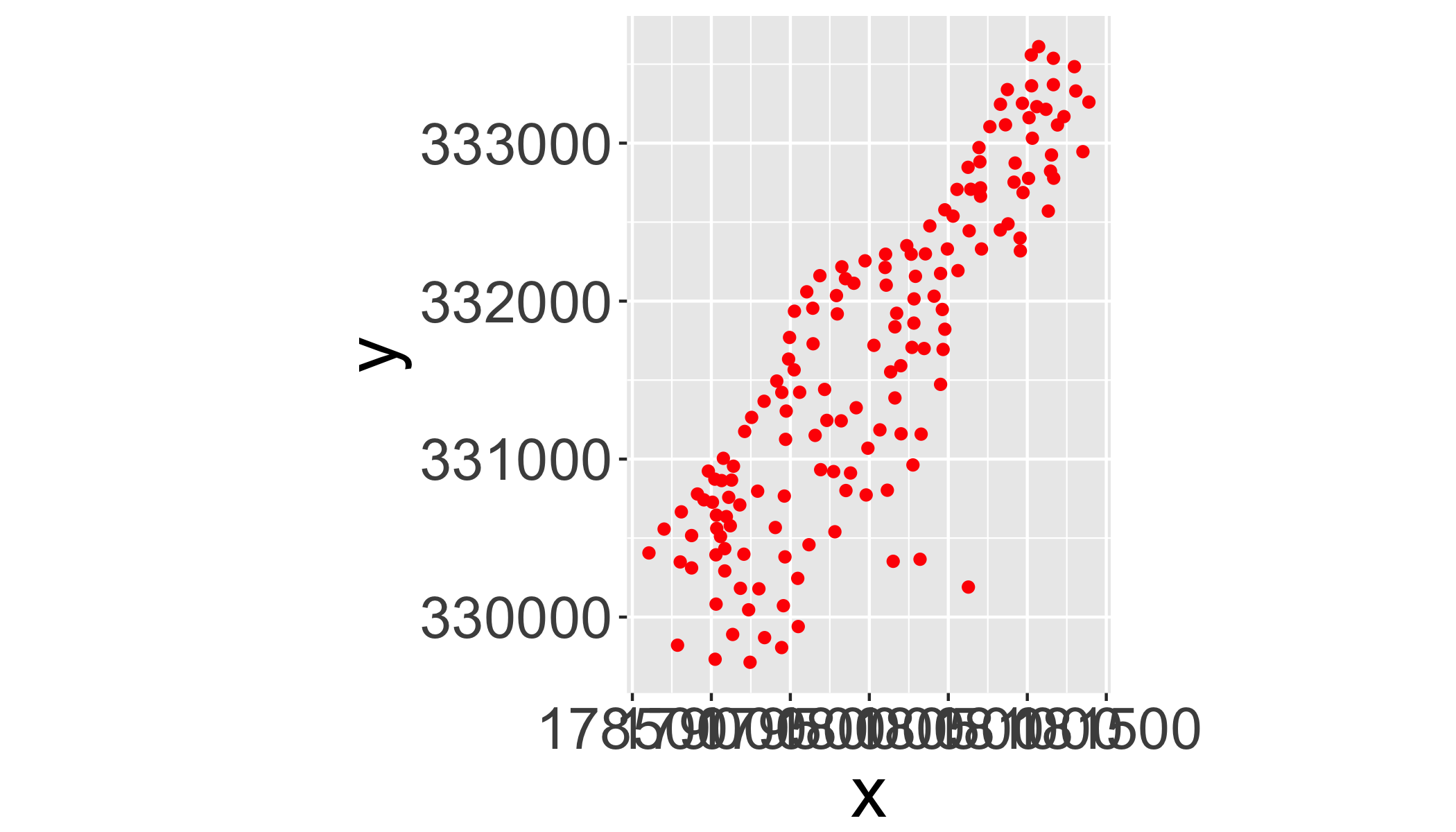

Note that ggplot works only with data.frames. Convert with as.data.frame() or fortify().

2.7 ggplot

If you’re not familiar with ggplot, here’s a quick digression. For a more detailed version, see the ggplot section in Lesson 03: Plotting. # ggplot2 The grammar of graphics consists of specifying a number of key elements of a plot. These are the same elements you’d put in any base graphics plot; this approach just provides a consisent way of defining them

Data: The raw data
geom_: The geometric shapes representing data (e.g. use a circle or triangle)
aes(): Aesthetics of the geometric and statistical objects (color, size, shape, and position)
scale_: Maps between the data and the aesthetic dimensions (e.g. x- and y-limits)

data
+ geometry,
+ aesthetic mappings like position, color and size
+ scaling of ranges of the data to ranges of the aesthetics

Additional settings

stat_: Statistical summaries of the data that can be plotted, such as quantiles, fitted curves (loess, linear models), etc.
coord_: Transformation for mapping data coordinates into the plane of the data rectangle
facet_: Arrangement of data into grid of plots (e.g. a grid with one plot for each species, location, or time)
theme: Visual defaults (background, grids, axes, typeface, colors, etc.)

# Old Faithful Geyser Data on duration and waiting times.
library("MASS")
data(geyser)
m <- ggplot(geyser, aes(x = duration, y = waiting)) # define data
m + # reference the data
  geom_point() +  # add points
  stat_density2d(geom="contour") + # add a contour plot
  xlim(0.5, 6) + ylim(40, 110) # define plot limits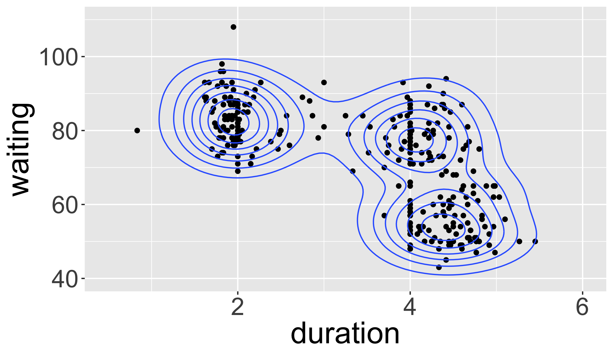

And now back to spatial data …

3 Raster Package

3.1 `getData()`

Raster package includes access to some useful (vector and raster) datasets with getData():

Elevation (SRTM 90m resolution raster)
World Climate (Tmin, Tmax, Precip, BioClim rasters)
Countries from CIA factsheet (vector!)
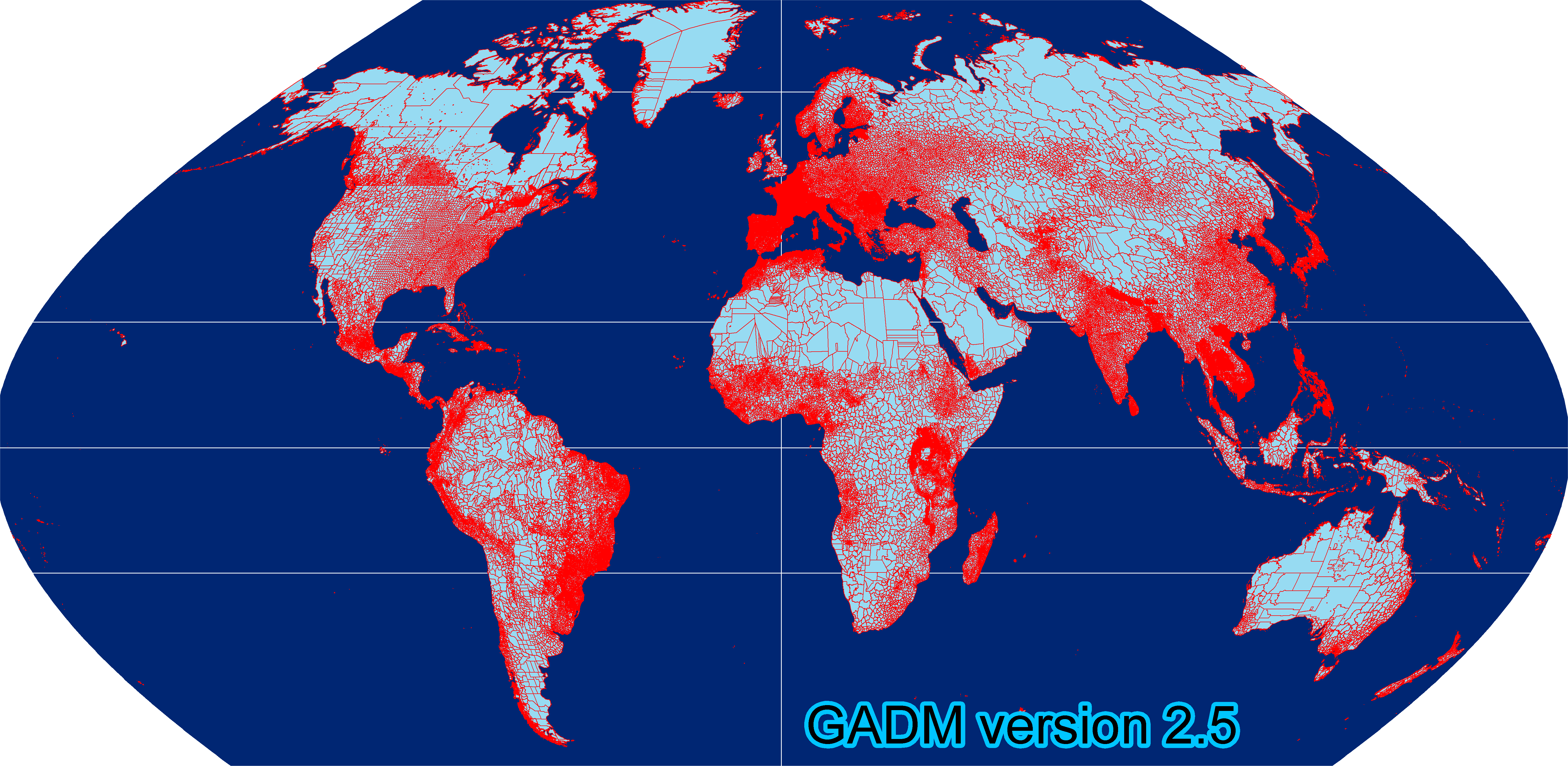
Global Administrative boundaries (vector!)

getData() steps for GADM:

Select Dataset: ‘GADM’ returns the global administrative boundaries.
Select country: Country name of the boundaries using its ISO A3 country code
Specify level: Level of of administrative subdivision (0=country, 1=first level subdivision).

3.2 GADM: Global Administrative Areas

Administrative areas in this database are countries and lower level subdivisions.

alt text

Divided by country (see website for full dataset). Explore country list:

getData("ISO3")%>%
  as.data.frame%>%
  filter(NAME=="South Africa")

##   ISO3         NAME
## 1  ZAF South Africa

Note that %>% is a pipe, defined by the dplyr package that says ’Use the previous thing as the first argument in this function. So this is equivalent to temp1 = getData("ISO3") followed by temp2 = as.data.frame(temp1) followed by output=filter(temp2,NAME==South Africa').

Download data for South Africa

za=getData('GADM', country='ZAF', level=1)

plot(za) # this can be a little slow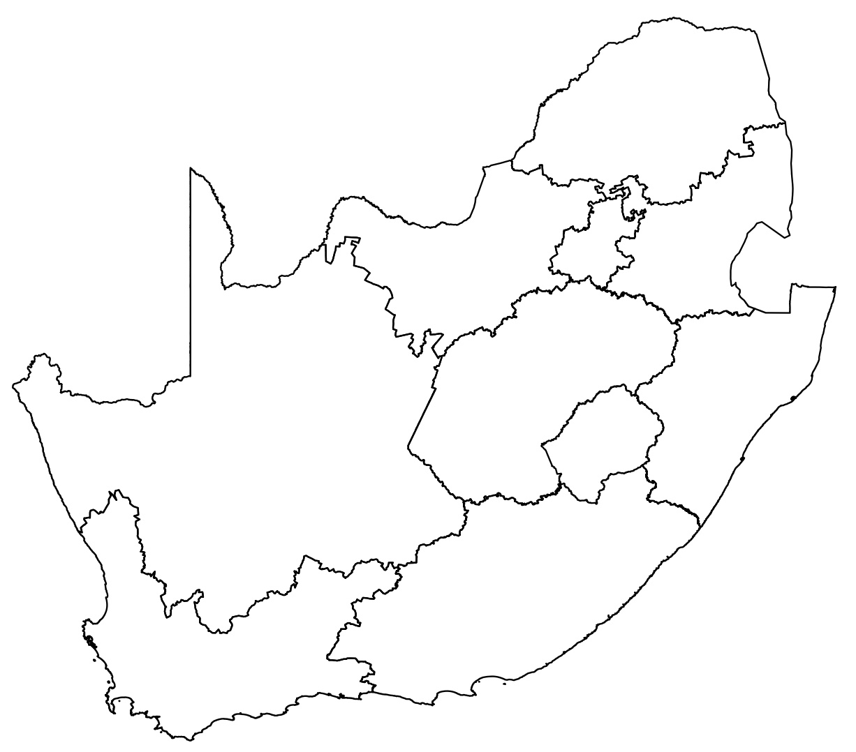

alt text

Danger: plot() works, but can be slow for complex polygons.

3.2.1 Check out attribute table

za@data

##   OBJECTID ID_0 ISO       NAME_0 ID_1        NAME_1 HASC_1 CCN_1 CCA_1
## 1        1  211 ZAF South Africa    1  Eastern Cape  ZA.EC    NA    EC
## 2        2  211 ZAF South Africa    2    Free State  ZA.FS    NA    FS
## 3        3  211 ZAF South Africa    3       Gauteng  ZA.GT    NA    GT
## 4        4  211 ZAF South Africa    4 KwaZulu-Natal  ZA.NL    NA   KZN
## 5        5  211 ZAF South Africa    5       Limpopo  ZA.NP    NA   LIM
## 6        6  211 ZAF South Africa    6    Mpumalanga  ZA.MP    NA    MP
## 7        7  211 ZAF South Africa    7    North West  ZA.NW    NA    NW
## 8        8  211 ZAF South Africa    8 Northern Cape  ZA.NC    NA    NC
## 9        9  211 ZAF South Africa    9  Western Cape  ZA.WC    NA    WC
##      TYPE_1 ENGTYPE_1 NL_NAME_1
## 1 Provinsie  Province          
## 2 Provinsie  Province          
## 3 Provinsie  Province          
## 4 Provinsie  Province          
## 5 Provinsie  Province          
## 6 Provinsie  Province          
## 7 Provinsie  Province          
## 8 Provinsie  Province          
## 9 Provinsie  Province          
##                                                   VARNAME_1
## 1                                                  Oos-Kaap
## 2                                Orange Free State|Vrystaat
## 3                               Pretoria/Witwatersrand/Vaal
## 4                                        Natal and Zululand
## 5 Noordelike Provinsie|Northern Transvaal|Northern Province
## 6                                         Eastern Transvaal
## 7                                       North-West|Noordwes
## 8                                                Noord-Kaap
## 9                                                  Wes-Kaap

za=subset(za,NAME_1=="Eastern Cape")
plot(za)

3.2.1 Your turn

Use the method above to download and plot the boundaries for a country of your choice.

getData("ISO3")%>%
  as.data.frame%>%
  filter(NAME=="Tunisia")

country=getData('GADM', country='TUN', level=1)
plot(country)

4 Raster Data

4.1 Raster introduction

Spatial data structure dividing region (‘grid’) into rectangles (’cells’ or ’pixels’) storing one or more values each.

Some examples from the Raster vignette by Robert J. Hijmans.

rasterLayer: 1 band
rasterStack: Multiple Bands
rasterBrick: Multiple Bands of same thing.

Normally, you’ll obtain rasters data by downloading it from somewhere (e.g. global climate data below), but to get a better understanding of rasters, let’s build one from scratch.

x <- raster()

## NOTE: rgdal::checkCRSArgs: no proj_defs.dat in PROJ.4 shared files

## class       : RasterLayer 
## dimensions  : 180, 360, 64800  (nrow, ncol, ncell)
## resolution  : 1, 1  (x, y)
## extent      : -180, 180, -90, 90  (xmin, xmax, ymin, ymax)
## coord. ref. : +proj=longlat +datum=WGS84 +ellps=WGS84 +towgs84=0,0,0

There are lots of slots to handle all the ways one might need to use a raster; fortunately you won’t have to dig into the majority of these.

str(x)

## Formal class 'RasterLayer' [package "raster"] with 12 slots
##   ..@ file    :Formal class '.RasterFile' [package "raster"] with 13 slots
##   .. .. ..@ name        : chr ""
##   .. .. ..@ datanotation: chr "FLT4S"
##   .. .. ..@ byteorder   : chr "little"
##   .. .. ..@ nodatavalue : num -Inf
##   .. .. ..@ NAchanged   : logi FALSE
##   .. .. ..@ nbands      : int 1
##   .. .. ..@ bandorder   : chr "BIL"
##   .. .. ..@ offset      : int 0
##   .. .. ..@ toptobottom : logi TRUE
##   .. .. ..@ blockrows   : int 0
##   .. .. ..@ blockcols   : int 0
##   .. .. ..@ driver      : chr ""
##   .. .. ..@ open        : logi FALSE
##   ..@ data    :Formal class '.SingleLayerData' [package "raster"] with 13 slots
##   .. .. ..@ values    : logi(0) 
##   .. .. ..@ offset    : num 0
##   .. .. ..@ gain      : num 1
##   .. .. ..@ inmemory  : logi FALSE
##   .. .. ..@ fromdisk  : logi FALSE
##   .. .. ..@ isfactor  : logi FALSE
##   .. .. ..@ attributes: list()
##   .. .. ..@ haveminmax: logi FALSE
##   .. .. ..@ min       : num Inf
##   .. .. ..@ max       : num -Inf
##   .. .. ..@ band      : int 1
##   .. .. ..@ unit      : chr ""
##   .. .. ..@ names     : chr ""
##   ..@ legend  :Formal class '.RasterLegend' [package "raster"] with 5 slots
##   .. .. ..@ type      : chr(0) 
##   .. .. ..@ values    : logi(0) 
##   .. .. ..@ color     : logi(0) 
##   .. .. ..@ names     : logi(0) 
##   .. .. ..@ colortable: logi(0) 
##   ..@ title   : chr(0) 
##   ..@ extent  :Formal class 'Extent' [package "raster"] with 4 slots
##   .. .. ..@ xmin: num -180
##   .. .. ..@ xmax: num 180
##   .. .. ..@ ymin: num -90
##   .. .. ..@ ymax: num 90
##   ..@ rotated : logi FALSE
##   ..@ rotation:Formal class '.Rotation' [package "raster"] with 2 slots
##   .. .. ..@ geotrans: num(0) 
##   .. .. ..@ transfun:function ()  
##   ..@ ncols   : int 360
##   ..@ nrows   : int 180
##   ..@ crs     :Formal class 'CRS' [package "sp"] with 1 slot
##   .. .. ..@ projargs: chr "+proj=longlat +datum=WGS84 +ellps=WGS84 +towgs84=0,0,0"
##   ..@ history : list()
##   ..@ z       : list()

The most useful functions for accessing slots are values() to get data values, extent() to get the bounding box, crs() to get the projection.

x <- raster(ncol=36, nrow=18, xmn=-1000, xmx=1000, ymn=-100, ymx=900)
res(x)

## [1] 55.55556 55.55556

res(x) <- 100
res(x)

## [1] 100 100

ncol(x)

## [1] 20

# change the numer of columns (affects resolution)
ncol(x) <- 18
ncol(x)

## [1] 18

res(x)

## [1] 111.1111 100.0000

4.2 Raster data storage

r <- raster(ncol=10, nrow=10)

## NOTE: rgdal::checkCRSArgs: no proj_defs.dat in PROJ.4 shared files

ncell(r)

## [1] 100

But it is an empty raster

hasValues(r)

## [1] FALSE

Use values() function:

values(r) <- 1:ncell(r)
hasValues(r)

## [1] TRUE

values(r)[1:10]

##  [1]  1  2  3  4  5  6  7  8  9 10

4.2 Your turn

Create and then plot a new raster with:

100 rows
50 columns
Fill it with random values (rnorm())

x=raster(nrow=100,ncol=50,vals=rnorm(100*50))

## NOTE: rgdal::checkCRSArgs: no proj_defs.dat in PROJ.4 shared files

# OR
x= raster(nrow=100,ncol=50)

## NOTE: rgdal::checkCRSArgs: no proj_defs.dat in PROJ.4 shared files

values(x)= rnorm(5000)

plot(x)

## NOTE: rgdal::checkCRSArgs: no proj_defs.dat in PROJ.4 shared files
## NOTE: rgdal::checkCRSArgs: no proj_defs.dat in PROJ.4 shared files
## NOTE: rgdal::checkCRSArgs: no proj_defs.dat in PROJ.4 shared files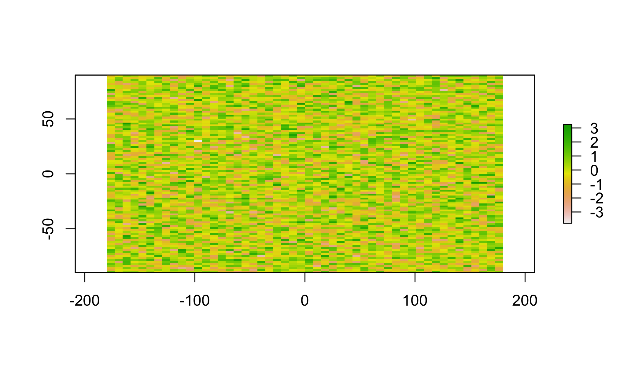

4.3 Raster memory usage

Raster data files can be very large, especially when cells are at high resolution, so it becomes important to think about how much RAM is required to work with a raster to avoid slowing your computer to a crawl. The raster package cleverly avoids reading full rasters into memory to instead just provides pointers to the relevant raster files.

inMemory(r)

## [1] TRUE

You can change the memory options using the maxmemory option in rasterOptions()

4.4 Raster Plotting

Plotting is easy (but slow) with plot.

plot(r, main='Raster with 100 cells')

## NOTE: rgdal::checkCRSArgs: no proj_defs.dat in PROJ.4 shared files
## NOTE: rgdal::checkCRSArgs: no proj_defs.dat in PROJ.4 shared files
## NOTE: rgdal::checkCRSArgs: no proj_defs.dat in PROJ.4 shared files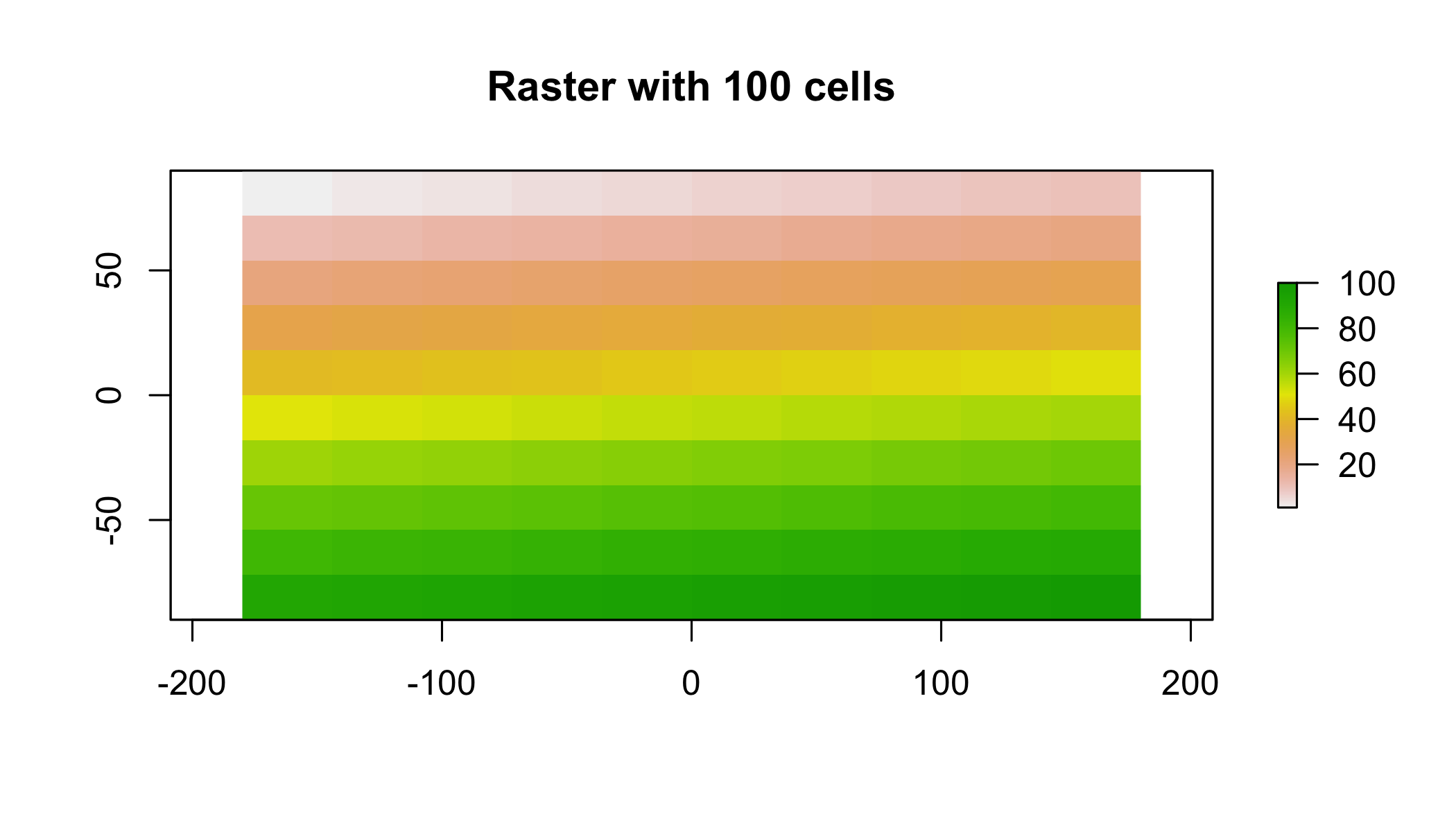

4.4.1 ggplot and rasterVis

rasterVis package has gplot() for plotting raster data in the ggplot() framework.

gplot(r,maxpixels=50000)+ # reference the data
  geom_raster(aes(fill=value)) # cell's data value determines its color

## NOTE: rgdal::checkCRSArgs: no proj_defs.dat in PROJ.4 shared files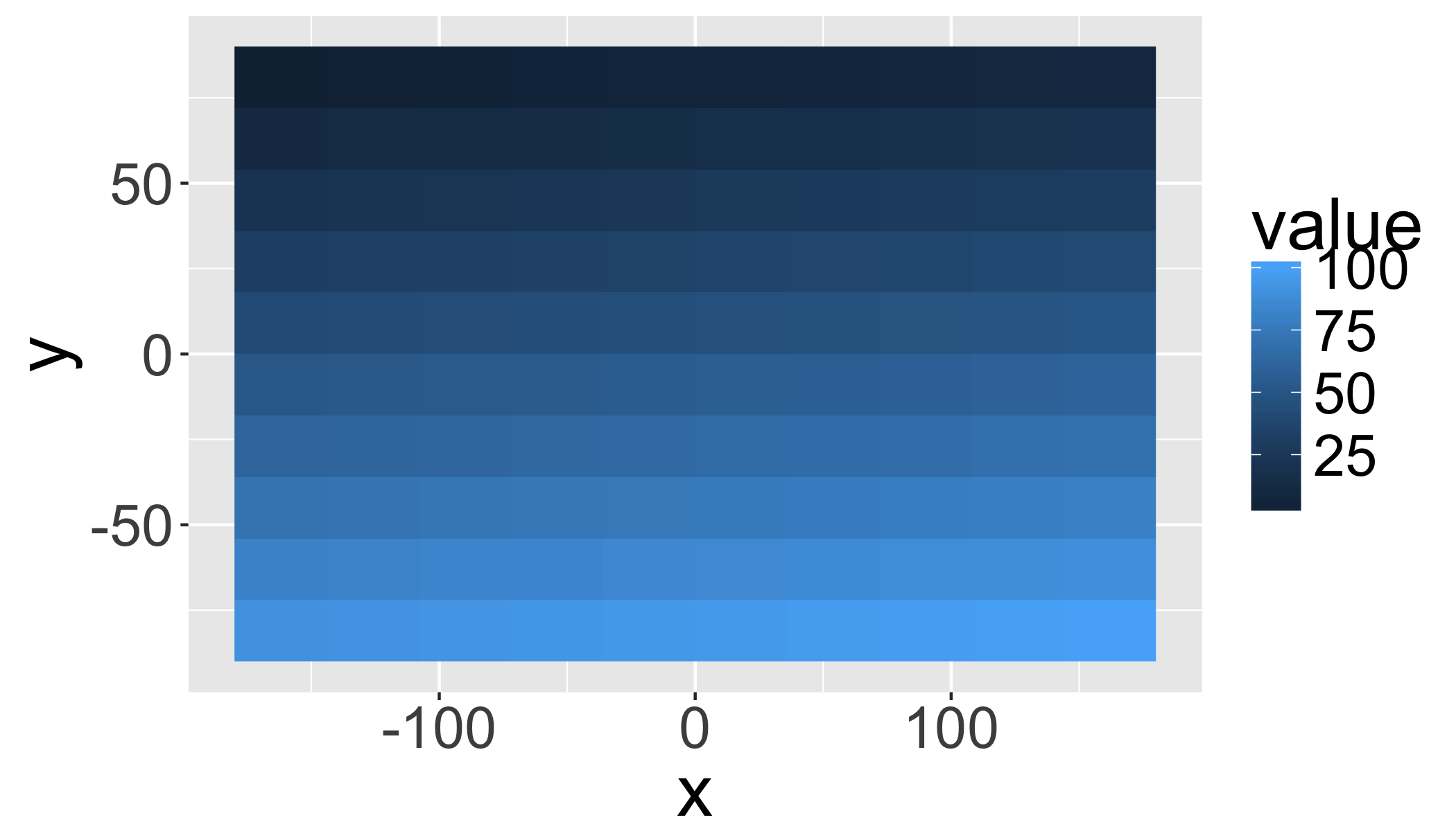

Adjust maxpixels for faster plotting of large datasets.

gplot(r,maxpixels=10)+
  geom_raster(aes(fill=value))

## NOTE: rgdal::checkCRSArgs: no proj_defs.dat in PROJ.4 shared files
## NOTE: rgdal::checkCRSArgs: no proj_defs.dat in PROJ.4 shared files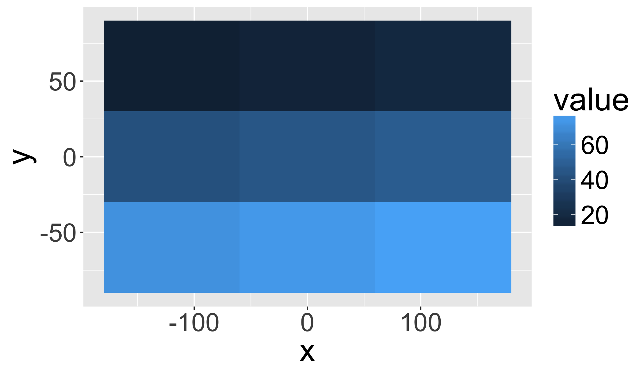

Can use all the ggplot color ramps, etc.

gplot(r)+ # reference the data
  geom_raster(aes(fill=value))+ # cell's data value determines its color
  scale_fill_distiller(palette="OrRd") # specify the color pallette

## NOTE: rgdal::checkCRSArgs: no proj_defs.dat in PROJ.4 shared files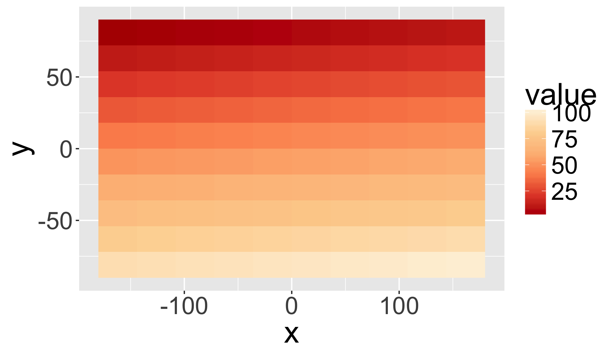

4.5 Spatial Projections

Raster package uses standard coordinate reference system (CRS).

For example, see the projection format for the standard WGS84.

projection(r)

## [1] "+proj=longlat +datum=WGS84 +ellps=WGS84 +towgs84=0,0,0"

5 WorldClim

5.1 Overview of WorldClim

Mean monthly climate and derived variables interpolated from weather stations on a 30 arc-second (~1km) grid. See worldclim.org

5.2 Bioclim variables

Varia	ble Description
BIO1	Annual Mean Temperature
BIO2	Mean Diurnal Range (Mean of monthly (max temp – min temp))
BIO3	Isothermality (BIO2/BIO7) (* 100)
BIO4	Temperature Seasonality (standard deviation *100)
BIO5	Max Temperature of Warmest Month
BIO6	Min Temperature of Coldest Month
BIO7	Temperature Annual Range (BIO5-BIO6)
BIO8	Mean Temperature of Wettest Quarter
BIO9	Mean Temperature of Driest Quarter
BIO10	Mean Temperature of Warmest Quarter
BIO11	Mean Temperature of Coldest Quarter
BIO12	Annual Precipitation
BIO13	Precipitation of Wettest Month
BIO14	Precipitation of Driest Month
BIO15	Precipitation Seasonality (Coefficient of Variation)
BIO16	Precipitation of Wettest Quarter
BIO17	Precipitation of Driest Quarter
BIO18	Precipitation of Warmest Quarter
BIO19	Precipitation of Coldest Quarter

5.3 Download climate data

Download the data:

clim=getData('worldclim', var='bio', res=10)

## NOTE: rgdal::checkCRSArgs: no proj_defs.dat in PROJ.4 shared files
## NOTE: rgdal::checkCRSArgs: no proj_defs.dat in PROJ.4 shared files
## NOTE: rgdal::checkCRSArgs: no proj_defs.dat in PROJ.4 shared files
## NOTE: rgdal::checkCRSArgs: no proj_defs.dat in PROJ.4 shared files
## NOTE: rgdal::checkCRSArgs: no proj_defs.dat in PROJ.4 shared files
## NOTE: rgdal::checkCRSArgs: no proj_defs.dat in PROJ.4 shared files
## NOTE: rgdal::checkCRSArgs: no proj_defs.dat in PROJ.4 shared files
## NOTE: rgdal::checkCRSArgs: no proj_defs.dat in PROJ.4 shared files
## NOTE: rgdal::checkCRSArgs: no proj_defs.dat in PROJ.4 shared files
## NOTE: rgdal::checkCRSArgs: no proj_defs.dat in PROJ.4 shared files
## NOTE: rgdal::checkCRSArgs: no proj_defs.dat in PROJ.4 shared files
## NOTE: rgdal::checkCRSArgs: no proj_defs.dat in PROJ.4 shared files
## NOTE: rgdal::checkCRSArgs: no proj_defs.dat in PROJ.4 shared files
## NOTE: rgdal::checkCRSArgs: no proj_defs.dat in PROJ.4 shared files
## NOTE: rgdal::checkCRSArgs: no proj_defs.dat in PROJ.4 shared files
## NOTE: rgdal::checkCRSArgs: no proj_defs.dat in PROJ.4 shared files
## NOTE: rgdal::checkCRSArgs: no proj_defs.dat in PROJ.4 shared files
## NOTE: rgdal::checkCRSArgs: no proj_defs.dat in PROJ.4 shared files
## NOTE: rgdal::checkCRSArgs: no proj_defs.dat in PROJ.4 shared files
## NOTE: rgdal::checkCRSArgs: no proj_defs.dat in PROJ.4 shared files
## NOTE: rgdal::checkCRSArgs: no proj_defs.dat in PROJ.4 shared files

res is resolution (0.5, 2.5, 5, and 10 minutes of a degree)

5.3.1 Gain and Offset

clim

## class       : RasterStack 
## dimensions  : 900, 2160, 1944000, 19  (nrow, ncol, ncell, nlayers)
## resolution  : 0.1666667, 0.1666667  (x, y)
## extent      : -180, 180, -60, 90  (xmin, xmax, ymin, ymax)
## coord. ref. : +proj=longlat +datum=WGS84 +ellps=WGS84 +towgs84=0,0,0 
## names       :  bio1,  bio2,  bio3,  bio4,  bio5,  bio6,  bio7,  bio8,  bio9, bio10, bio11, bio12, bio13, bio14, bio15, ... 
## min values  :  -269,     9,     8,    72,   -59,  -547,    53,  -251,  -450,   -97,  -488,     0,     0,     0,     0, ... 
## max values  :   314,   211,    95, 22673,   489,   258,   725,   375,   364,   380,   289,  9916,  2088,   652,   261, ...

Note the min/max of the raster. What are the units? Always check metadata, the WorldClim temperature dataset has a gain of 0.1, meaning that it must be multipled by 0.1 to convert back to degrees Celsius. Precipitation is in mm, so a gain of 0.1 would turn that into cm.

gain(clim)=0.1

5.3.2 Plot with `plot()`

plot(clim[[1:3]]) # just the first 3, since its slow

## NOTE: rgdal::checkCRSArgs: no proj_defs.dat in PROJ.4 shared files
## NOTE: rgdal::checkCRSArgs: no proj_defs.dat in PROJ.4 shared files
## NOTE: rgdal::checkCRSArgs: no proj_defs.dat in PROJ.4 shared files
## NOTE: rgdal::checkCRSArgs: no proj_defs.dat in PROJ.4 shared files
## NOTE: rgdal::checkCRSArgs: no proj_defs.dat in PROJ.4 shared files
## NOTE: rgdal::checkCRSArgs: no proj_defs.dat in PROJ.4 shared files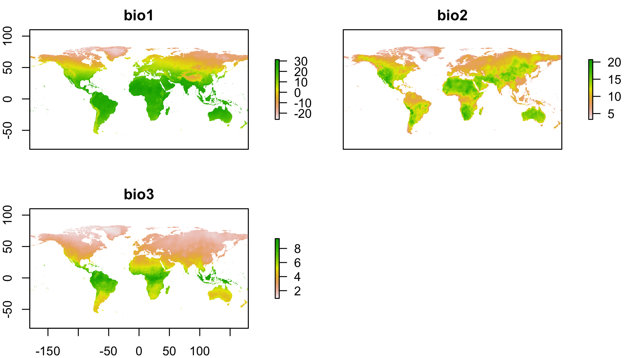

5.4 Faceting in ggplot

Or use rasterVis methods with gplot

gplot(clim[[1:3]])+geom_raster(aes(fill=value))+
  facet_wrap(~variable)+
  scale_fill_gradientn(colours=c("brown","red","yellow","darkgreen","green"),trans="log10")+
  coord_equal()

## NOTE: rgdal::checkCRSArgs: no proj_defs.dat in PROJ.4 shared files
## NOTE: rgdal::checkCRSArgs: no proj_defs.dat in PROJ.4 shared files
## NOTE: rgdal::checkCRSArgs: no proj_defs.dat in PROJ.4 shared files

## Warning in self$trans$transform(x): NaNs produced

## Warning: Transformation introduced infinite values in discrete y-axis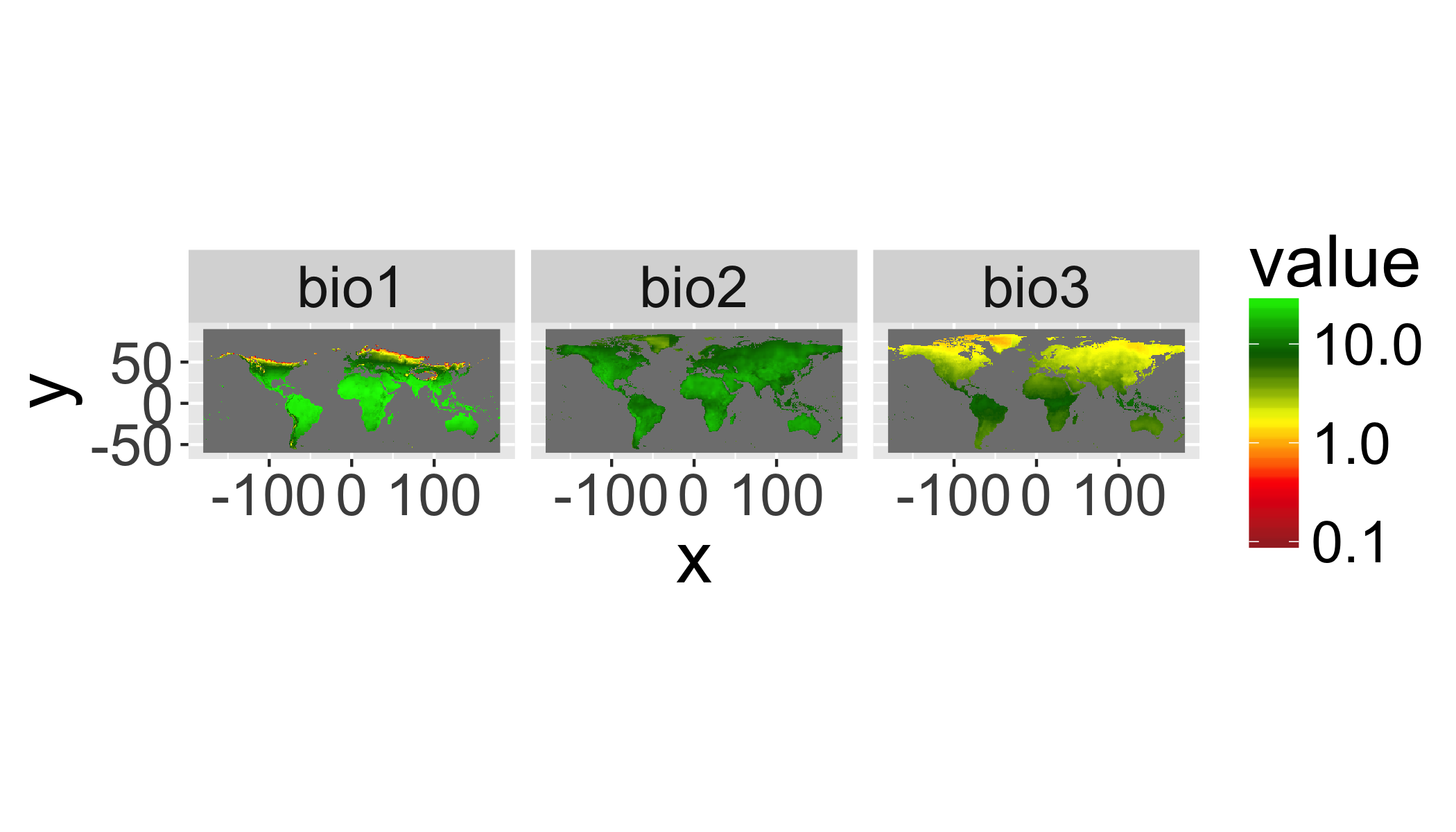

Let’s dig a little deeper into the data object:

## is it held in RAM?
inMemory(clim)

## [1] FALSE

## How big is it?
object.size(clim)

## 227920 bytes

## can we work with it directly in RAM?
canProcessInMemory(clim)

## [1] TRUE

5.5 Subsetting and spatial cropping

Use [[1:3]] to select raster layers from raster stack.

## crop to a latitude/longitude box
r1 <- crop(clim[[1]], extent(10,35,-35,-20))

## NOTE: rgdal::checkCRSArgs: no proj_defs.dat in PROJ.4 shared files

## Crop using a Spatial polygon
r1 <- crop(clim[[1]], bbox(za))

## NOTE: rgdal::checkCRSArgs: no proj_defs.dat in PROJ.4 shared files

r1

## class       : RasterLayer 
## dimensions  : 76, 98, 7448  (nrow, ncol, ncell)
## resolution  : 0.1666667, 0.1666667  (x, y)
## extent      : 16.5, 32.83333, -34.83333, -22.16667  (xmin, xmax, ymin, ymax)
## coord. ref. : +proj=longlat +datum=WGS84 +ellps=WGS84 +towgs84=0,0,0 
## data source : in memory
## names       : bio1 
## values      : 5.8, 24.6  (min, max)

plot(r1)

## NOTE: rgdal::checkCRSArgs: no proj_defs.dat in PROJ.4 shared files
## NOTE: rgdal::checkCRSArgs: no proj_defs.dat in PROJ.4 shared files
## NOTE: rgdal::checkCRSArgs: no proj_defs.dat in PROJ.4 shared files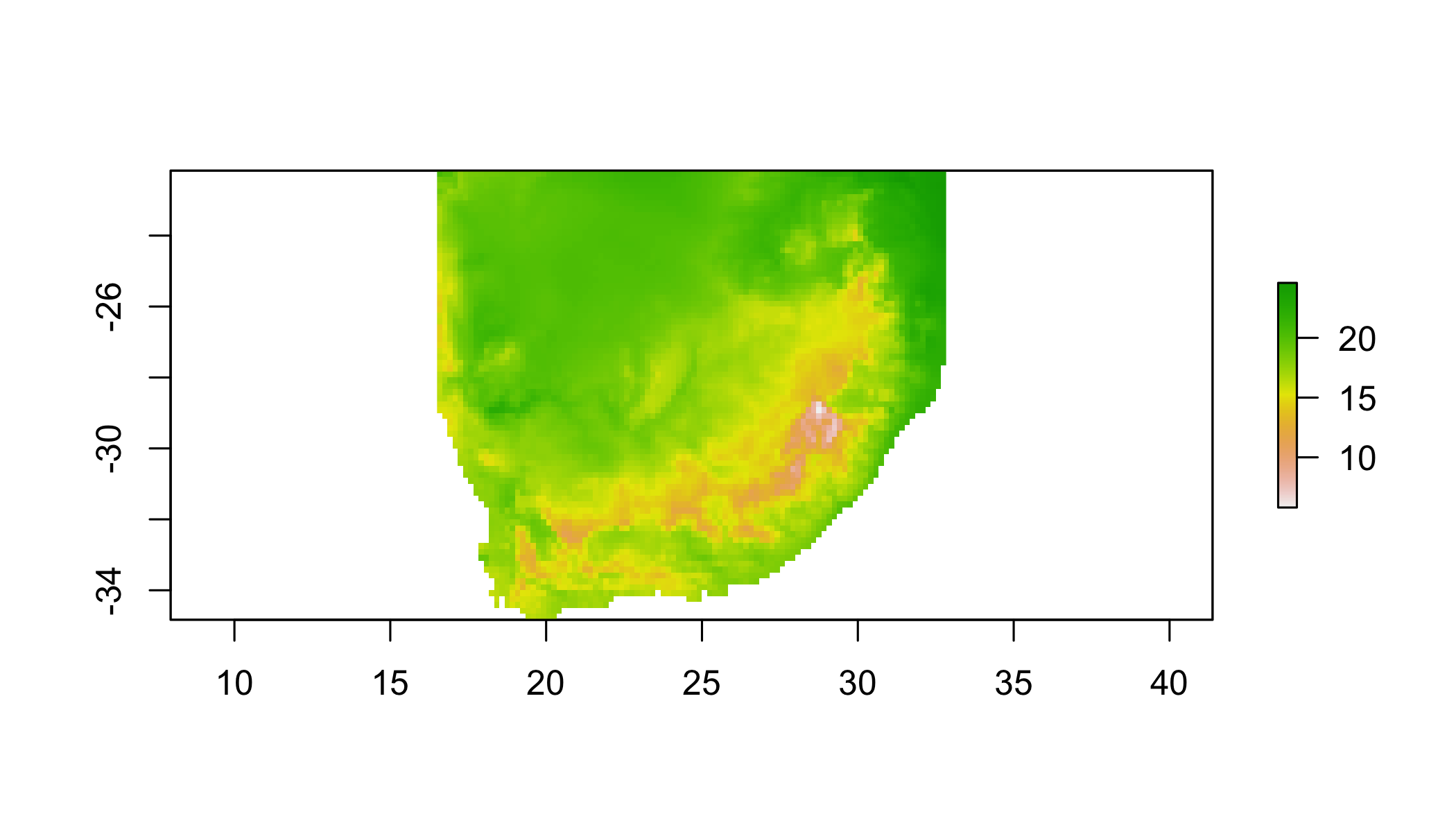

5.6 Spatial aggregation

## aggregate using a function
aggregate(r1, 3, fun=mean) %>%
  plot()

## NOTE: rgdal::checkCRSArgs: no proj_defs.dat in PROJ.4 shared files
## NOTE: rgdal::checkCRSArgs: no proj_defs.dat in PROJ.4 shared files
## NOTE: rgdal::checkCRSArgs: no proj_defs.dat in PROJ.4 shared files
## NOTE: rgdal::checkCRSArgs: no proj_defs.dat in PROJ.4 shared files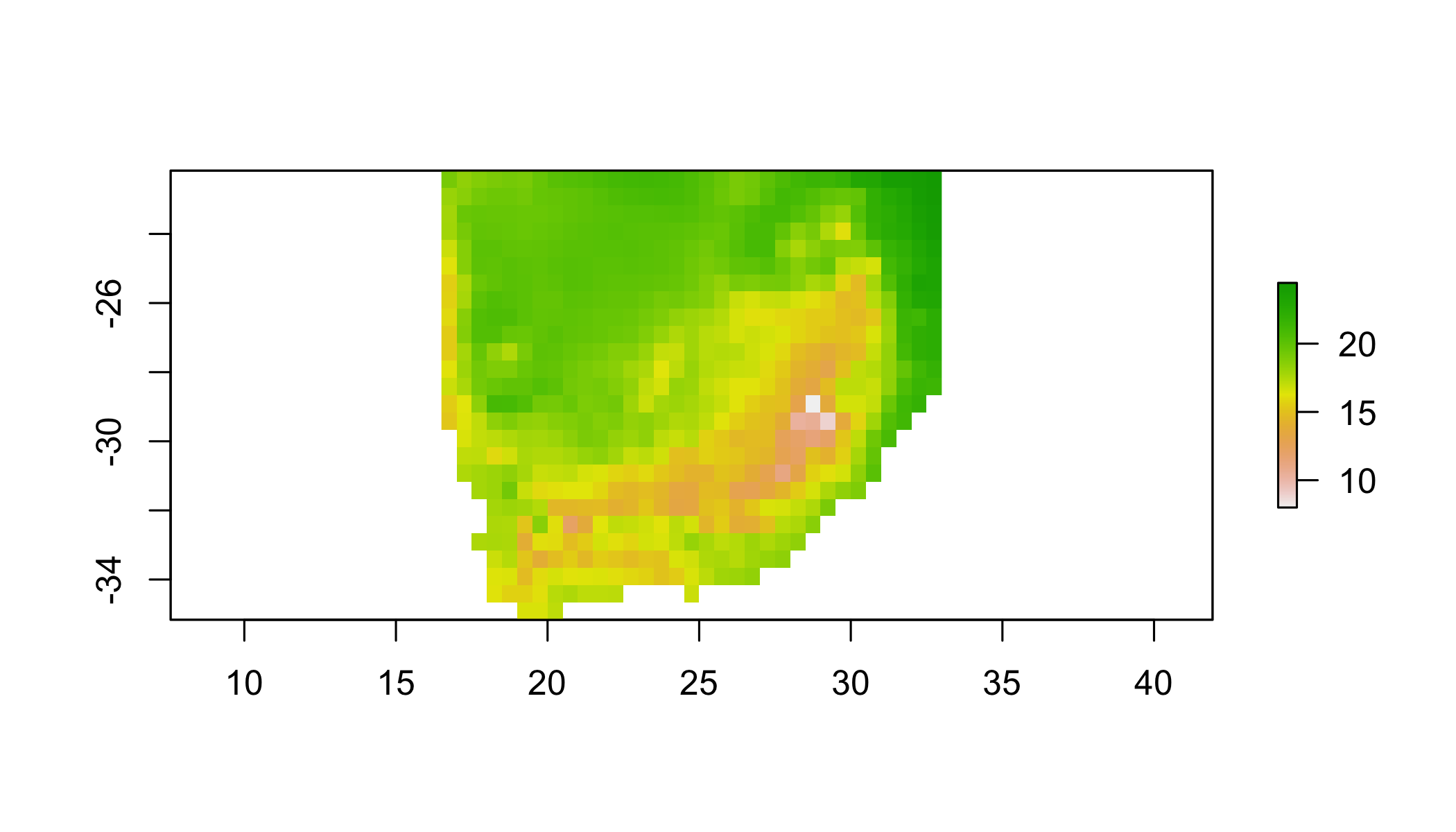

5.6 Your turn

Create a new raster by aggregating to the minimum (min) value of r1 within a 10 pixel window

aggregate(r1, 10, fun=min) %>%
  plot()

## NOTE: rgdal::checkCRSArgs: no proj_defs.dat in PROJ.4 shared files
## NOTE: rgdal::checkCRSArgs: no proj_defs.dat in PROJ.4 shared files
## NOTE: rgdal::checkCRSArgs: no proj_defs.dat in PROJ.4 shared files
## NOTE: rgdal::checkCRSArgs: no proj_defs.dat in PROJ.4 shared files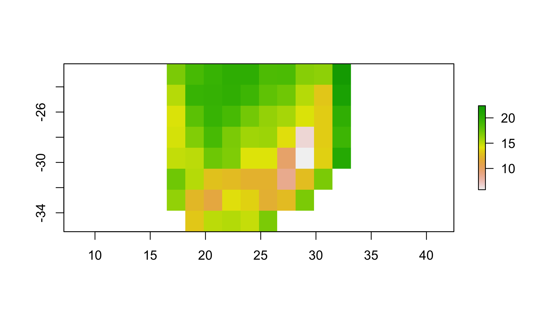

5.7 Focal (“moving window”)

## apply a function over a moving window
focal(r1, w=matrix(1,3,3), fun=mean) %>% 
  plot()

## NOTE: rgdal::checkCRSArgs: no proj_defs.dat in PROJ.4 shared files
## NOTE: rgdal::checkCRSArgs: no proj_defs.dat in PROJ.4 shared files
## NOTE: rgdal::checkCRSArgs: no proj_defs.dat in PROJ.4 shared files
## NOTE: rgdal::checkCRSArgs: no proj_defs.dat in PROJ.4 shared files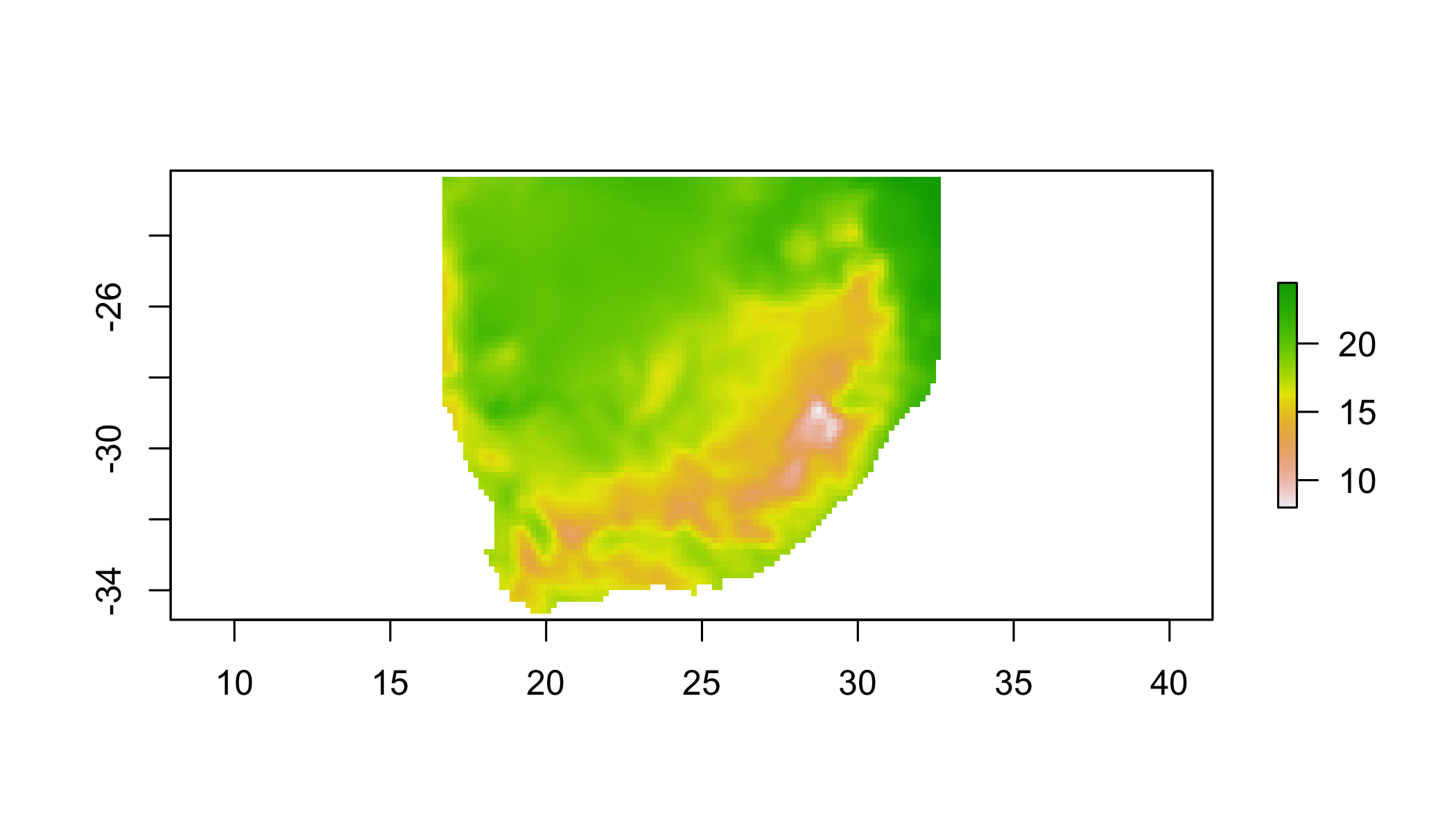

## apply a function over a moving window
rf_min <- focal(r1, w=matrix(1,11,11), fun=min)

## NOTE: rgdal::checkCRSArgs: no proj_defs.dat in PROJ.4 shared files

rf_max <- focal(r1, w=matrix(1,11,11), fun=max)

## NOTE: rgdal::checkCRSArgs: no proj_defs.dat in PROJ.4 shared files

rf_range=rf_max-rf_min

## NOTE: rgdal::checkCRSArgs: no proj_defs.dat in PROJ.4 shared files

## or just use the range function
rf_range2 <- focal(r1, w=matrix(1,11,11), fun=range)

## NOTE: rgdal::checkCRSArgs: no proj_defs.dat in PROJ.4 shared files

plot(rf_range2)

## NOTE: rgdal::checkCRSArgs: no proj_defs.dat in PROJ.4 shared files
## NOTE: rgdal::checkCRSArgs: no proj_defs.dat in PROJ.4 shared files
## NOTE: rgdal::checkCRSArgs: no proj_defs.dat in PROJ.4 shared files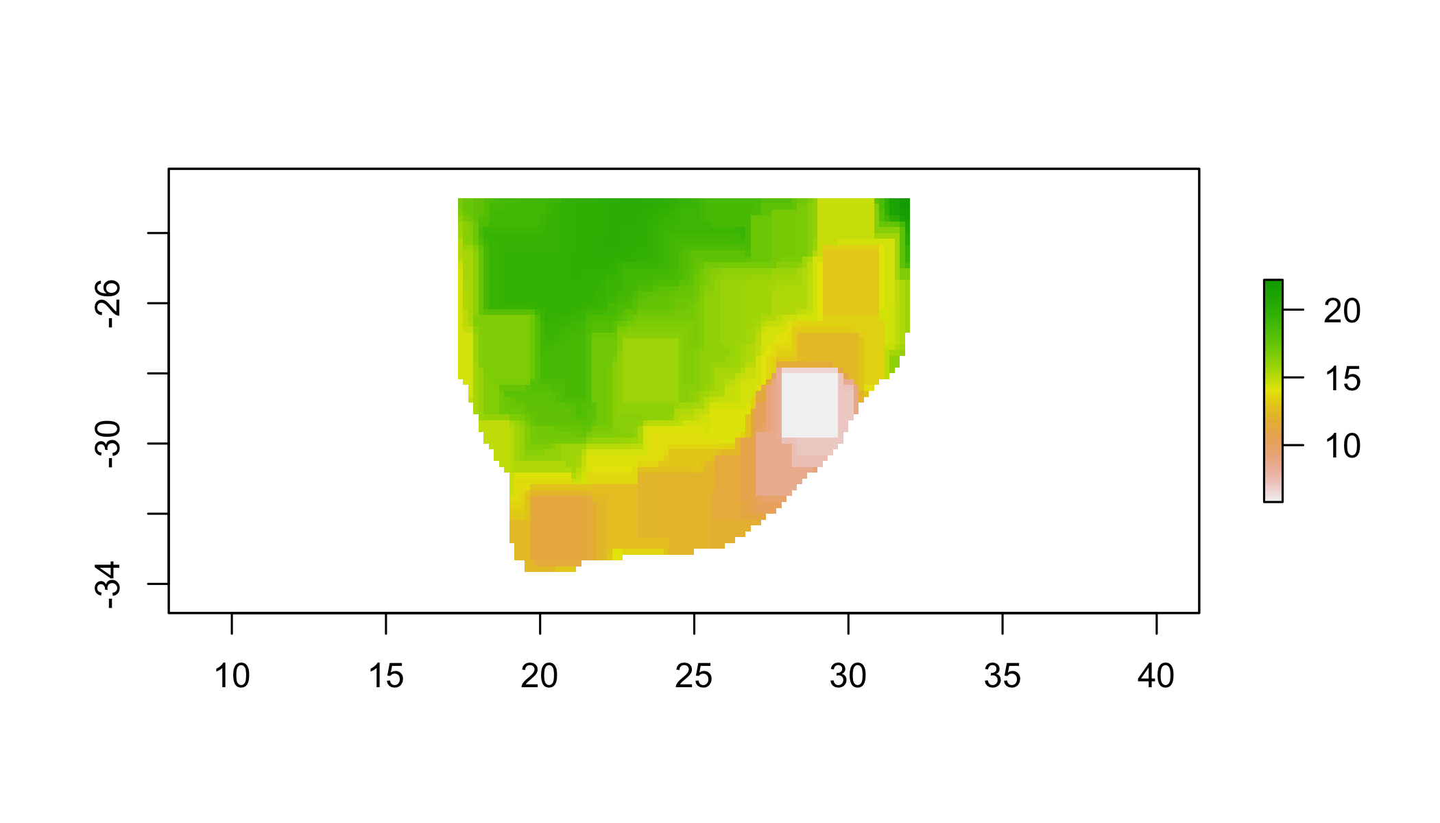

5.7 Your turn

Plot the focal standard deviation of r1 over a 3x3 window.

focal(r1,w=matrix(1,3,3),fun=sd)%>%
  plot()

## NOTE: rgdal::checkCRSArgs: no proj_defs.dat in PROJ.4 shared files
## NOTE: rgdal::checkCRSArgs: no proj_defs.dat in PROJ.4 shared files
## NOTE: rgdal::checkCRSArgs: no proj_defs.dat in PROJ.4 shared files
## NOTE: rgdal::checkCRSArgs: no proj_defs.dat in PROJ.4 shared files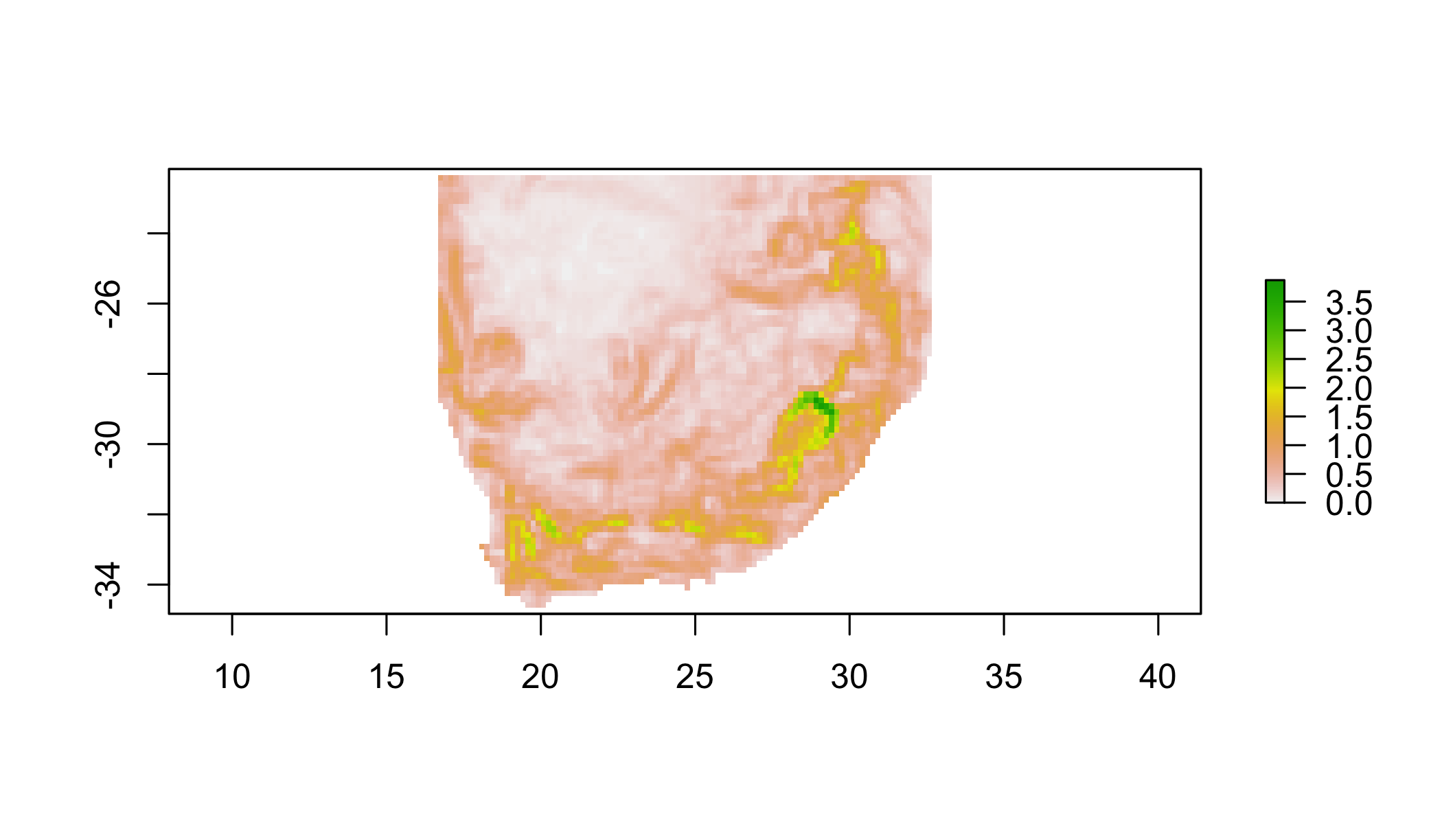

5.8 Raster calculations

The raster package has many options for raster algebra, including +, -, *, /, logical operators such as >, >=, <, ==, ! and functions such as abs, round, ceiling, floor, trunc, sqrt, log, log10, exp, cos, sin, max, min, range, prod, sum, any, all.

So, for example, you can

cellStats(r1,range)

## [1]  5.8 24.6

## add 10
s = r1 + 10

## NOTE: rgdal::checkCRSArgs: no proj_defs.dat in PROJ.4 shared files

cellStats(s,range)

## [1] 15.8 34.6

## take the square root
s = sqrt(r1)

## NOTE: rgdal::checkCRSArgs: no proj_defs.dat in PROJ.4 shared files

cellStats(s,range)

## [1] 2.408319 4.959839

# round values
r = round(r1)

## NOTE: rgdal::checkCRSArgs: no proj_defs.dat in PROJ.4 shared files

cellStats(r,range)

## [1]  6 25

# find cells with values less than 15 degrees C
r = r1 < 15

## NOTE: rgdal::checkCRSArgs: no proj_defs.dat in PROJ.4 shared files

plot(r)

## NOTE: rgdal::checkCRSArgs: no proj_defs.dat in PROJ.4 shared files
## NOTE: rgdal::checkCRSArgs: no proj_defs.dat in PROJ.4 shared files
## NOTE: rgdal::checkCRSArgs: no proj_defs.dat in PROJ.4 shared files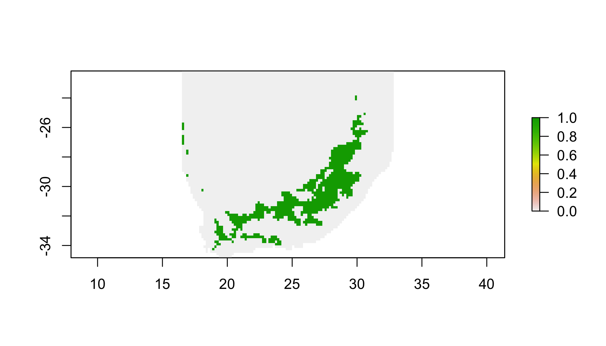

5.8.1 Apply algebraic functions

# multiply s times r and add 5
s = s * r1 + 5

## NOTE: rgdal::checkCRSArgs: no proj_defs.dat in PROJ.4 shared files
## NOTE: rgdal::checkCRSArgs: no proj_defs.dat in PROJ.4 shared files

cellStats(s,range)

## [1]  18.96825 127.01203

5.9 Extracting Raster Data

points
lines
polygons
extent (rectangle)
cell numbers

Extract all intersecting values OR apply a summarizing function with fun.

5.9.1 Point data

sampleRandom() generates random points and automatically extracts the raster values for those points. Also check out ?sampleStratified and sampleRegular().

Generate 100 random points and the associated climate variables at those points.

## define a new dataset of points to play with
pts=sampleRandom(clim,100,xy=T,sp=T)

## NOTE: rgdal::checkCRSArgs: no proj_defs.dat in PROJ.4 shared files

plot(pts);axis(1);axis(2)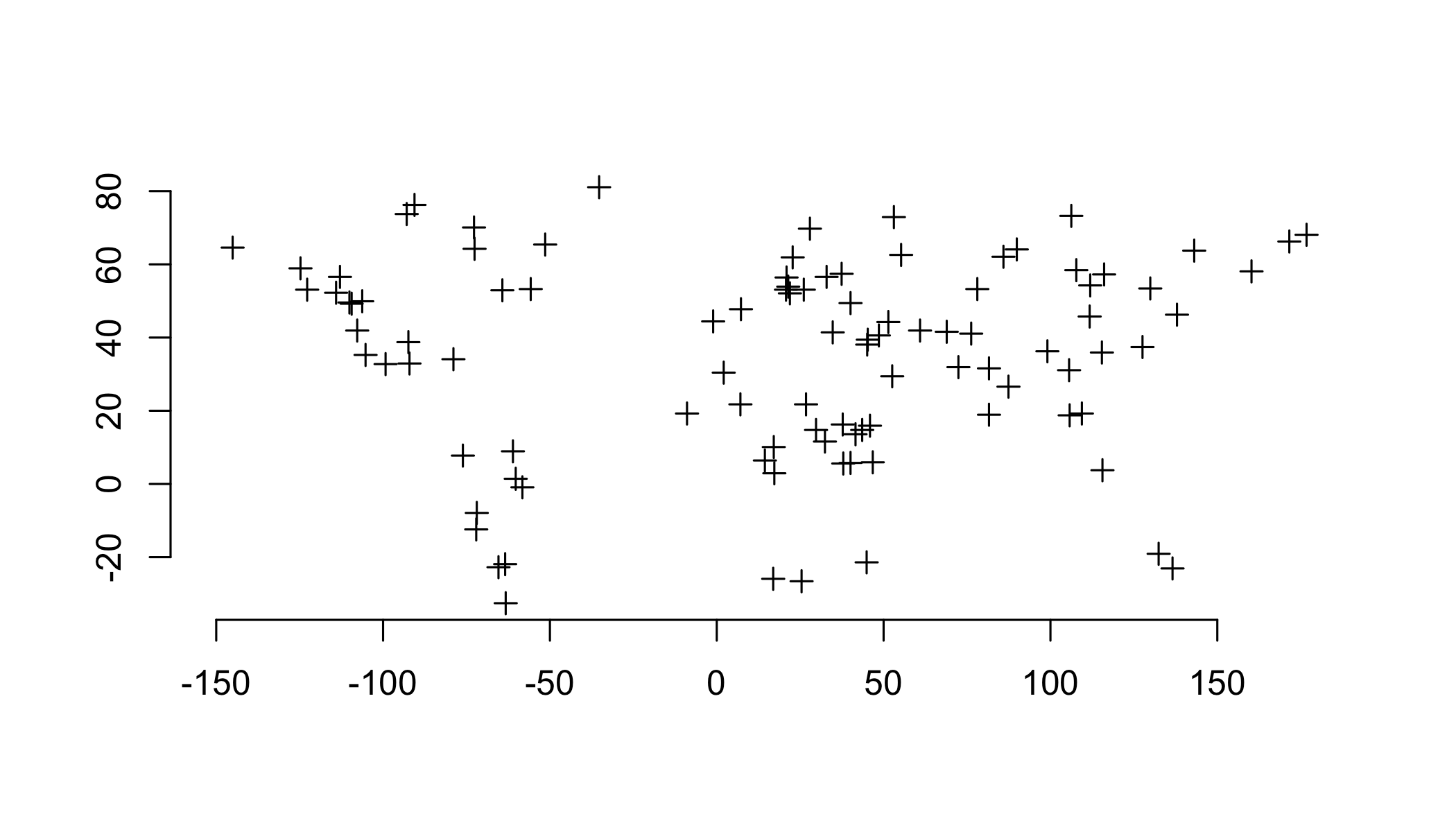

5.9.2 Extract data using a `SpatialPoints` object

Often you will have some locations (points) for which you want data from a raster* object. You can use the extract function here with the pts object (we’ll pretend it’s a new point dataset for which you want climate variables).

pts_data=raster::extract(clim[[1:4]],pts,df=T)

## NOTE: rgdal::checkCRSArgs: no proj_defs.dat in PROJ.4 shared files
## NOTE: rgdal::checkCRSArgs: no proj_defs.dat in PROJ.4 shared files
## NOTE: rgdal::checkCRSArgs: no proj_defs.dat in PROJ.4 shared files
## NOTE: rgdal::checkCRSArgs: no proj_defs.dat in PROJ.4 shared files
## NOTE: rgdal::checkCRSArgs: no proj_defs.dat in PROJ.4 shared files
## NOTE: rgdal::checkCRSArgs: no proj_defs.dat in PROJ.4 shared files
## NOTE: rgdal::checkCRSArgs: no proj_defs.dat in PROJ.4 shared files
## NOTE: rgdal::checkCRSArgs: no proj_defs.dat in PROJ.4 shared files

head(pts_data)

##   ID bio1 bio2 bio3   bio4
## 1  1 12.7 12.6  2.8 1114.2
## 2  2  3.1  8.4  2.5  838.5
## 3  3 23.0 11.6  7.0   90.5
## 4  4  2.9 15.2  3.1 1098.9
## 5  5 11.8  8.7  3.2  642.8
## 6  6 23.7 13.4  6.2  259.9

Use package::function to avoid confusion with similar functions.

5.9.3 Plot the global dataset with the random points

gplot(clim[[1]])+
  geom_raster(aes(fill=value))+
  geom_point(
    data=as.data.frame(pts),
    aes(x=x,y=y),col="red")+
  coord_equal()

## NOTE: rgdal::checkCRSArgs: no proj_defs.dat in PROJ.4 shared files
## NOTE: rgdal::checkCRSArgs: no proj_defs.dat in PROJ.4 shared files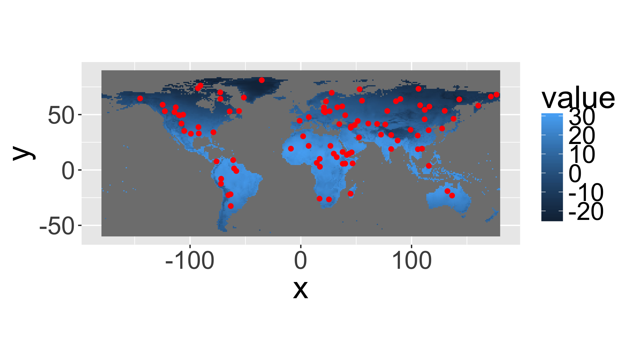

5.9.4 Summarize climate data at point locations

Use gather() to reshape the climate data for easy plotting with ggplot.

d2=pts_data%>%
  gather(ID)
colnames(d2)[1]="cell"
head(d2)

##   cell   ID value
## 1    1 bio1  12.7
## 2    2 bio1   3.1
## 3    3 bio1  23.0
## 4    4 bio1   2.9
## 5    5 bio1  11.8
## 6    6 bio1  23.7

And plot density plots (like histograms).

ggplot(d2,aes(x=value))+
  geom_density()+
  facet_wrap(~ID,scales="free")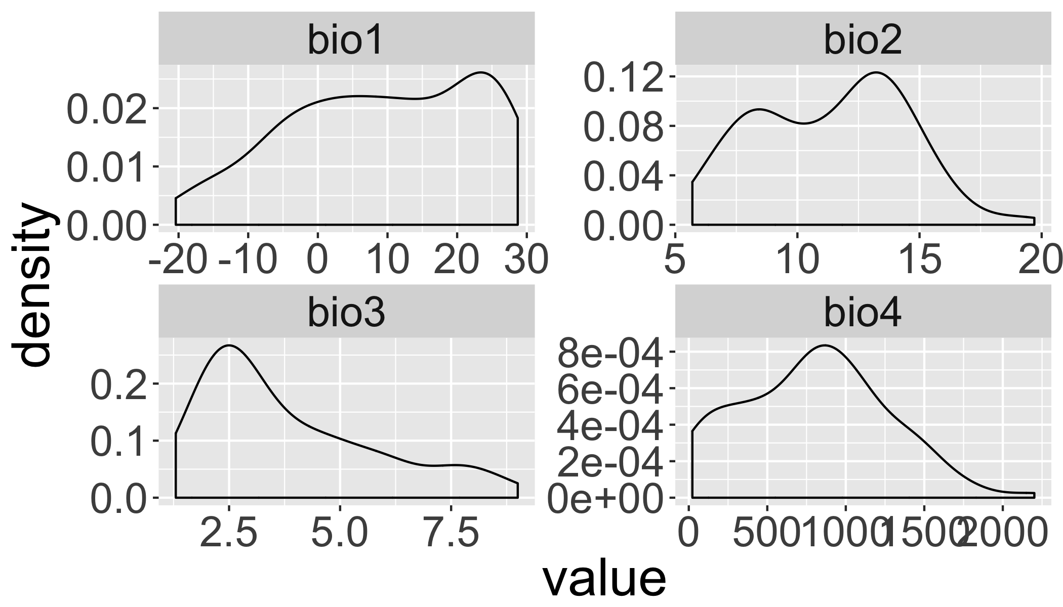

5.9.5 Lines

Extract values along a transect.

transect = SpatialLinesDataFrame(
  SpatialLines(list(Lines(list(Line(
    rbind(c(19, -33.5),c(26, -33.5)))), ID = "ZAF"))),
  data.frame(Z = c("transect"), row.names = c("ZAF")))

# OR

transect=SpatialLinesDataFrame(
  readWKT("LINESTRING(19 -33.5,26 -33.5)"),
  data.frame(Z = c("transect")))


gplot(r1)+geom_tile(aes(fill=value))+
  geom_line(aes(x=long,y=lat),data=fortify(transect),col="red")

## NOTE: rgdal::checkCRSArgs: no proj_defs.dat in PROJ.4 shared files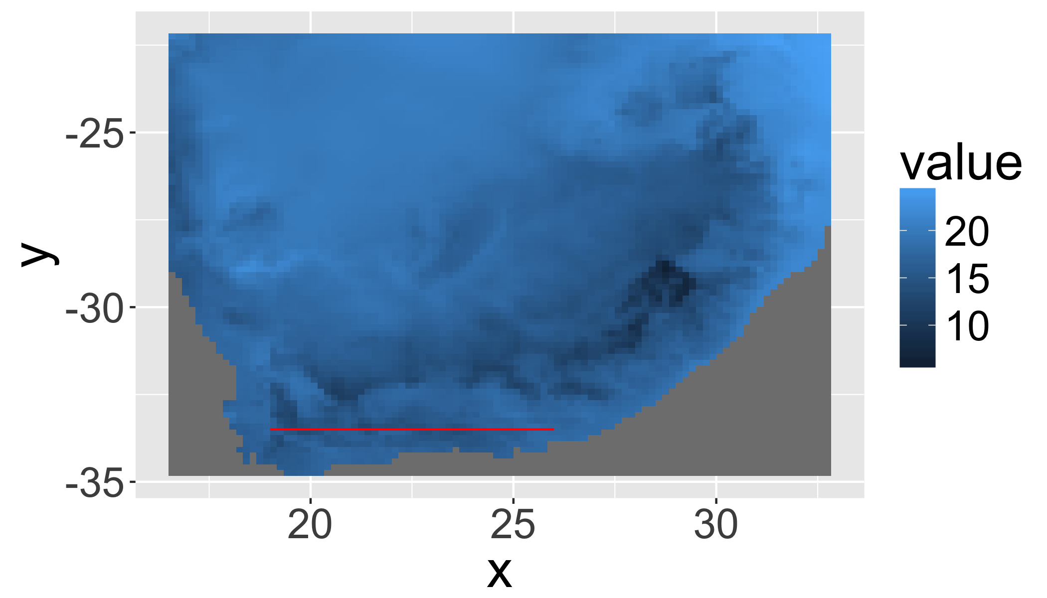

5.9.6 Plot Transect

trans=raster::extract(x=clim[[12:14]],
                      y=transect,
                      along=T,
                      cellnumbers=T)%>%
  data.frame()

## NOTE: rgdal::checkCRSArgs: no proj_defs.dat in PROJ.4 shared files
## NOTE: rgdal::checkCRSArgs: no proj_defs.dat in PROJ.4 shared files
## NOTE: rgdal::checkCRSArgs: no proj_defs.dat in PROJ.4 shared files
## NOTE: rgdal::checkCRSArgs: no proj_defs.dat in PROJ.4 shared files
## NOTE: rgdal::checkCRSArgs: no proj_defs.dat in PROJ.4 shared files
## NOTE: rgdal::checkCRSArgs: no proj_defs.dat in PROJ.4 shared files
## NOTE: rgdal::checkCRSArgs: no proj_defs.dat in PROJ.4 shared files
## NOTE: rgdal::checkCRSArgs: no proj_defs.dat in PROJ.4 shared files
## NOTE: rgdal::checkCRSArgs: no proj_defs.dat in PROJ.4 shared files

head(trans)

##      cell bio12 bio13 bio14
## 1 1601755  81.4  13.0   2.0
## 2 1601756  71.9  11.6   1.7
## 3 1601757  56.8   8.8   1.5
## 4 1601758  47.9   7.2   1.3
## 5 1601759  41.5   6.1   1.3
## 6 1601760  36.1   5.0   1.2

5.9.6.1 Add other metadata and reshape

trans[,c("lon","lat")]=coordinates(clim)[trans$cell]
trans$order=as.integer(rownames(trans))
head(trans)

##      cell bio12 bio13 bio14      lon      lat order
## 1 1601755  81.4  13.0   2.0 19.08333 19.08333     1
## 2 1601756  71.9  11.6   1.7 19.25000 19.25000     2
## 3 1601757  56.8   8.8   1.5 19.41667 19.41667     3
## 4 1601758  47.9   7.2   1.3 19.58333 19.58333     4
## 5 1601759  41.5   6.1   1.3 19.75000 19.75000     5
## 6 1601760  36.1   5.0   1.2 19.91667 19.91667     6

transl=group_by(trans,lon,lat)%>%
  gather(variable, value, -lon, -lat, -cell, -order)
head(transl)

## Source: local data frame [6 x 6]
## Groups: lon, lat [6]
## 
##      cell      lon      lat order variable value
##     <dbl>    <dbl>    <dbl> <int>    <chr> <dbl>
## 1 1601755 19.08333 19.08333     1    bio12  81.4
## 2 1601756 19.25000 19.25000     2    bio12  71.9
## 3 1601757 19.41667 19.41667     3    bio12  56.8
## 4 1601758 19.58333 19.58333     4    bio12  47.9
## 5 1601759 19.75000 19.75000     5    bio12  41.5
## 6 1601760 19.91667 19.91667     6    bio12  36.1

ggplot(transl,aes(x=lon,y=value,
                  colour=variable,
                  group=variable,
                  order=order))+
  geom_line()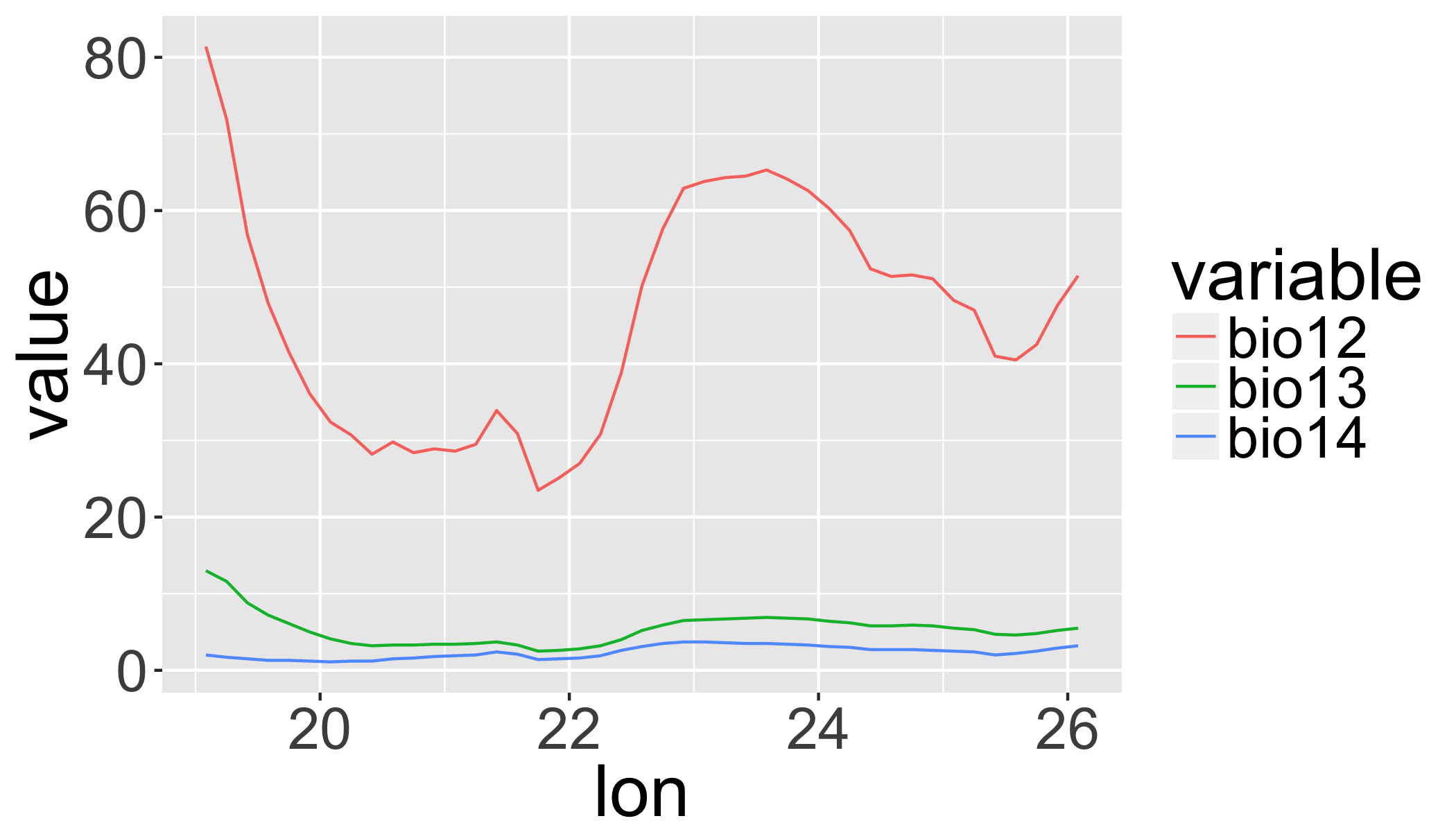

5.9.7 Zonal statistics

Calculate mean annual temperature averaged by province (polygons).

rsp=raster::extract(x=r1,
                    y=za,
                    fun=mean,
                    sp=T)

## NOTE: rgdal::checkCRSArgs: no proj_defs.dat in PROJ.4 shared files
## NOTE: rgdal::checkCRSArgs: no proj_defs.dat in PROJ.4 shared files
## NOTE: rgdal::checkCRSArgs: no proj_defs.dat in PROJ.4 shared files
## NOTE: rgdal::checkCRSArgs: no proj_defs.dat in PROJ.4 shared files
## NOTE: rgdal::checkCRSArgs: no proj_defs.dat in PROJ.4 shared files
## NOTE: rgdal::checkCRSArgs: no proj_defs.dat in PROJ.4 shared files
## NOTE: rgdal::checkCRSArgs: no proj_defs.dat in PROJ.4 shared files
## NOTE: rgdal::checkCRSArgs: no proj_defs.dat in PROJ.4 shared files
## NOTE: rgdal::checkCRSArgs: no proj_defs.dat in PROJ.4 shared files
## NOTE: rgdal::checkCRSArgs: no proj_defs.dat in PROJ.4 shared files
## NOTE: rgdal::checkCRSArgs: no proj_defs.dat in PROJ.4 shared files
## NOTE: rgdal::checkCRSArgs: no proj_defs.dat in PROJ.4 shared files
## NOTE: rgdal::checkCRSArgs: no proj_defs.dat in PROJ.4 shared files
## NOTE: rgdal::checkCRSArgs: no proj_defs.dat in PROJ.4 shared files
## NOTE: rgdal::checkCRSArgs: no proj_defs.dat in PROJ.4 shared files
## NOTE: rgdal::checkCRSArgs: no proj_defs.dat in PROJ.4 shared files
## NOTE: rgdal::checkCRSArgs: no proj_defs.dat in PROJ.4 shared files
## NOTE: rgdal::checkCRSArgs: no proj_defs.dat in PROJ.4 shared files
## NOTE: rgdal::checkCRSArgs: no proj_defs.dat in PROJ.4 shared files
## NOTE: rgdal::checkCRSArgs: no proj_defs.dat in PROJ.4 shared files
## NOTE: rgdal::checkCRSArgs: no proj_defs.dat in PROJ.4 shared files
## NOTE: rgdal::checkCRSArgs: no proj_defs.dat in PROJ.4 shared files
## NOTE: rgdal::checkCRSArgs: no proj_defs.dat in PROJ.4 shared files
## NOTE: rgdal::checkCRSArgs: no proj_defs.dat in PROJ.4 shared files
## NOTE: rgdal::checkCRSArgs: no proj_defs.dat in PROJ.4 shared files
## NOTE: rgdal::checkCRSArgs: no proj_defs.dat in PROJ.4 shared files
## NOTE: rgdal::checkCRSArgs: no proj_defs.dat in PROJ.4 shared files
## NOTE: rgdal::checkCRSArgs: no proj_defs.dat in PROJ.4 shared files

#spplot(rsp,zcol="bio1")

## add the ID to the dataframe itself for easier indexing in the map
rsp$id=as.numeric(rownames(rsp@data))
## create fortified version for plotting with ggplot()
frsp=fortify(rsp,region="id")

ggplot(rsp@data, aes(map_id = id, fill=bio1)) +
    expand_limits(x = frsp$long, y = frsp$lat)+
    scale_fill_gradientn(
      colours = c("grey","goldenrod","darkgreen","green"))+
    coord_map()+
    geom_map(map = frsp)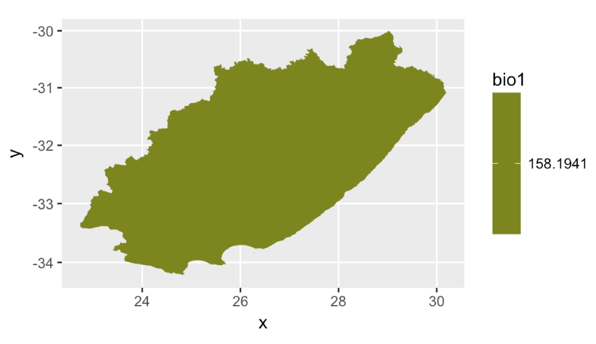

alt text

Not a very exciting plot, but then again, we did just ask for the mean value across the province. For more details about plotting spatialPolygons, see here

5.10 Example Workflow

Download the Maximum Temperature dataset using getData()
Set the gain to 0.1 (to convert to degrees Celcius)
Crop it to the country you downloaded (or ZA?)
Calculate the overall range for each variable with cellStats()
Calculate the focal median with an 11x11 window with focal()
Create a transect across the region and extract the temperature data.

country=getData('GADM', country='TUN', level=1)
tmax=getData('worldclim', var='tmax', res=10)

## NOTE: rgdal::checkCRSArgs: no proj_defs.dat in PROJ.4 shared files
## NOTE: rgdal::checkCRSArgs: no proj_defs.dat in PROJ.4 shared files
## NOTE: rgdal::checkCRSArgs: no proj_defs.dat in PROJ.4 shared files
## NOTE: rgdal::checkCRSArgs: no proj_defs.dat in PROJ.4 shared files
## NOTE: rgdal::checkCRSArgs: no proj_defs.dat in PROJ.4 shared files
## NOTE: rgdal::checkCRSArgs: no proj_defs.dat in PROJ.4 shared files
## NOTE: rgdal::checkCRSArgs: no proj_defs.dat in PROJ.4 shared files
## NOTE: rgdal::checkCRSArgs: no proj_defs.dat in PROJ.4 shared files
## NOTE: rgdal::checkCRSArgs: no proj_defs.dat in PROJ.4 shared files
## NOTE: rgdal::checkCRSArgs: no proj_defs.dat in PROJ.4 shared files
## NOTE: rgdal::checkCRSArgs: no proj_defs.dat in PROJ.4 shared files
## NOTE: rgdal::checkCRSArgs: no proj_defs.dat in PROJ.4 shared files
## NOTE: rgdal::checkCRSArgs: no proj_defs.dat in PROJ.4 shared files
## NOTE: rgdal::checkCRSArgs: no proj_defs.dat in PROJ.4 shared files

gain(tmax)=0.1
names(tmax)

##  [1] "tmax1"  "tmax2"  "tmax3"  "tmax4"  "tmax5"  "tmax6"  "tmax7" 
##  [8] "tmax8"  "tmax9"  "tmax10" "tmax11" "tmax12"

Default layer names can be problematic/undesirable.

sort(names(tmax))

##  [1] "tmax1"  "tmax10" "tmax11" "tmax12" "tmax2"  "tmax3"  "tmax4" 
##  [8] "tmax5"  "tmax6"  "tmax7"  "tmax8"  "tmax9"

## Options
month.name

##  [1] "January"   "February"  "March"     "April"     "May"      
##  [6] "June"      "July"      "August"    "September" "October"  
## [11] "November"  "December"

month.abb

##  [1] "Jan" "Feb" "Mar" "Apr" "May" "Jun" "Jul" "Aug" "Sep" "Oct" "Nov"
## [12] "Dec"

sprintf("%02d",1:12)

##  [1] "01" "02" "03" "04" "05" "06" "07" "08" "09" "10" "11" "12"

sprintf("%04d",1:12)

##  [1] "0001" "0002" "0003" "0004" "0005" "0006" "0007" "0008" "0009" "0010"
## [11] "0011" "0012"

See ?sprintf for details

names(tmax)=sprintf("%02d",1:12)

tmax_crop=crop(tmax,country)

## NOTE: rgdal::checkCRSArgs: no proj_defs.dat in PROJ.4 shared files

tmaxave_crop=mean(tmax_crop)  # calculate mean annual maximum temperature

## NOTE: rgdal::checkCRSArgs: no proj_defs.dat in PROJ.4 shared files

tmaxavefocal_crop=focal(tmaxave_crop,
                        fun=median,
                        w=matrix(1,11,11))

## NOTE: rgdal::checkCRSArgs: no proj_defs.dat in PROJ.4 shared files

Only a few datasets are available usig getData() in the raster package, but you can download almost any file on the web with file.download().

Report quantiles for each layer in a raster* object

cellStats(tmax_crop,"quantile")

##       X01  X02  X03  X04  X05  X06  X07  X08  X09  X10  X11  X12
## 0%    8.4 10.1 13.8 17.4 21.9 26.4 29.6 30.3 26.6 19.7 14.1  9.6
## 25%  14.1 15.8 18.3 21.3 25.7 30.4 34.6 34.0 30.3 25.3 20.2 15.4
## 50%  15.3 17.4 21.0 25.0 28.9 33.3 36.4 35.8 32.8 27.6 21.7 16.6
## 75%  16.3 19.0 23.0 27.4 31.9 36.4 39.7 39.0 35.3 29.0 22.4 17.4
## 100% 18.1 21.2 25.6 31.2 35.9 41.4 43.3 42.6 38.5 31.9 24.5 18.9

5.11 Create a Transect (SpatialLinesDataFrame)

transect=SpatialLinesDataFrame(
  readWKT("LINESTRING(8 36,10 36)"),
  data.frame(Z = c("T1")))

5.12 Plot the timeseries of climate data

gplot(tmax_crop)+
  geom_tile(aes(fill=value))+
  scale_fill_gradientn(
    colours=c("brown","red","yellow","darkgreen","green"),
    name="Temp")+
  facet_wrap(~variable)+
  ## now add country overlays
  geom_path(data=fortify(country),
            mapping=aes(x=long,y=lat,
                        group=group,
                        order=order))+
  # now add transect line
  geom_line(aes(x=long,y=lat),
            data=fortify(transect),col="red",size=3)+
  coord_map()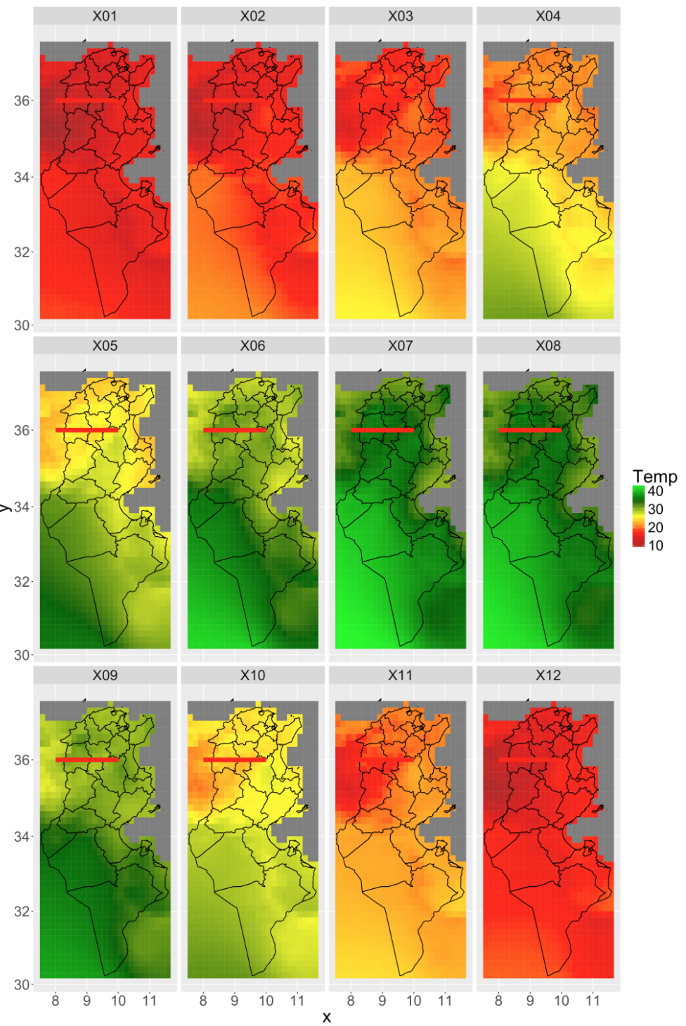

alt text

5.13 Extract and clean up the transect data

trans=raster::extract(tmax_crop,
                      transect,
                      along=T,
                      cellnumbers=T)%>% 
  as.data.frame()

## NOTE: rgdal::checkCRSArgs: no proj_defs.dat in PROJ.4 shared files
## NOTE: rgdal::checkCRSArgs: no proj_defs.dat in PROJ.4 shared files
## NOTE: rgdal::checkCRSArgs: no proj_defs.dat in PROJ.4 shared files

trans[,c("lon","lat")]=coordinates(tmax_crop)[trans$cell]
trans$order=as.integer(rownames(trans))
head(trans)

##   cell  X01  X02  X03  X04  X05  X06  X07  X08  X09  X10  X11  X12
## 1  229 12.0 13.3 16.7 20.4 24.5 30.4 34.5 33.9 29.4 23.0 17.3 13.0
## 2  230 12.6 14.1 17.4 21.1 25.3 31.4 35.5 34.9 30.3 23.8 18.0 13.8
## 3  231 12.8 14.3 17.6 21.3 25.6 31.8 36.1 35.4 30.7 24.1 18.2 14.0
## 4  232 11.8 13.3 16.8 20.6 25.0 31.1 35.7 34.8 30.0 23.4 17.4 13.1
## 5  233 11.6 13.1 16.6 20.4 25.0 30.9 35.7 34.7 29.9 23.3 17.4 13.0
## 6  234 11.3 12.7 16.3 20.0 24.8 30.5 35.4 34.4 29.6 23.2 17.3 12.8
##        lon      lat order
## 1 8.083333 8.083333     1
## 2 8.250000 8.250000     2
## 3 8.416667 8.416667     3
## 4 8.583333 8.583333     4
## 5 8.750000 8.750000     5
## 6 8.916667 8.916667     6

Reformat to ‘long’ format.

transl=group_by(trans,lon,lat)%>%
  gather(variable, value, -lon, -lat, -cell, -order)%>%
  separate(variable,into = c("X","month"),1)%>%
  mutate(month=as.numeric(month),monthname=factor(month.name[month],ordered=T,levels=month.name))
head(transl)

## Source: local data frame [6 x 8]
## Groups: lon, lat [6]
## 
##    cell      lon      lat order     X month value monthname
##   <dbl>    <dbl>    <dbl> <int> <chr> <dbl> <dbl>     <ord>
## 1   229 8.083333 8.083333     1     X     1  12.0   January
## 2   230 8.250000 8.250000     2     X     1  12.6   January
## 3   231 8.416667 8.416667     3     X     1  12.8   January
## 4   232 8.583333 8.583333     4     X     1  11.8   January
## 5   233 8.750000 8.750000     5     X     1  11.6   January
## 6   234 8.916667 8.916667     6     X     1  11.3   January

5.14 Plot the transect data

ggplot(transl,
       aes(x=lon,y=value,
           colour=month,
           group=month,
           order=order))+
  ylab("Maximum Temp")+
    scale_color_gradientn(
      colors=c("blue","green","red"),
      name="Month")+
    geom_line()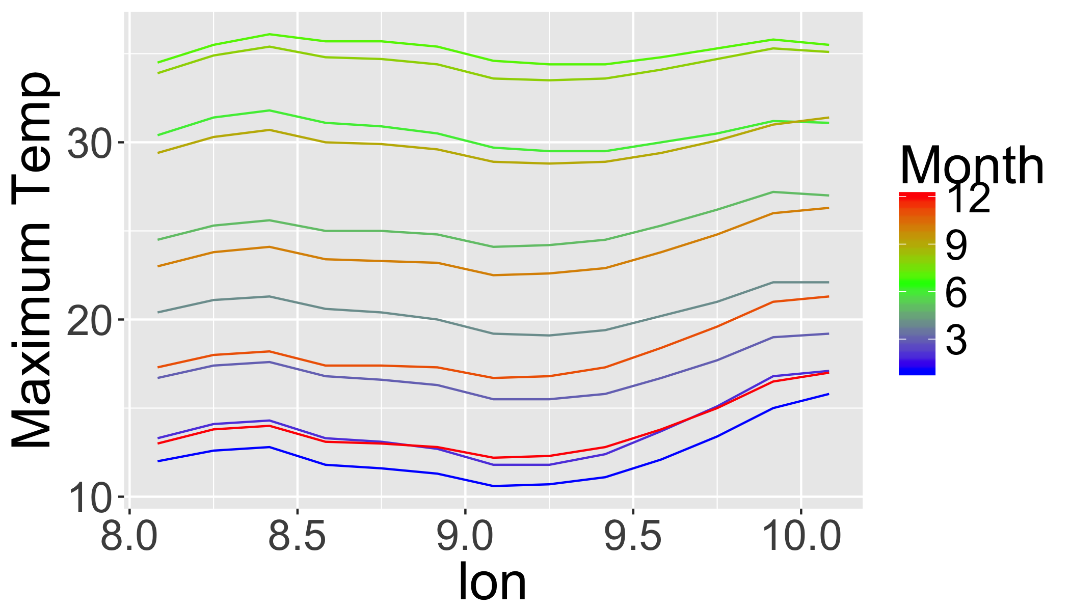

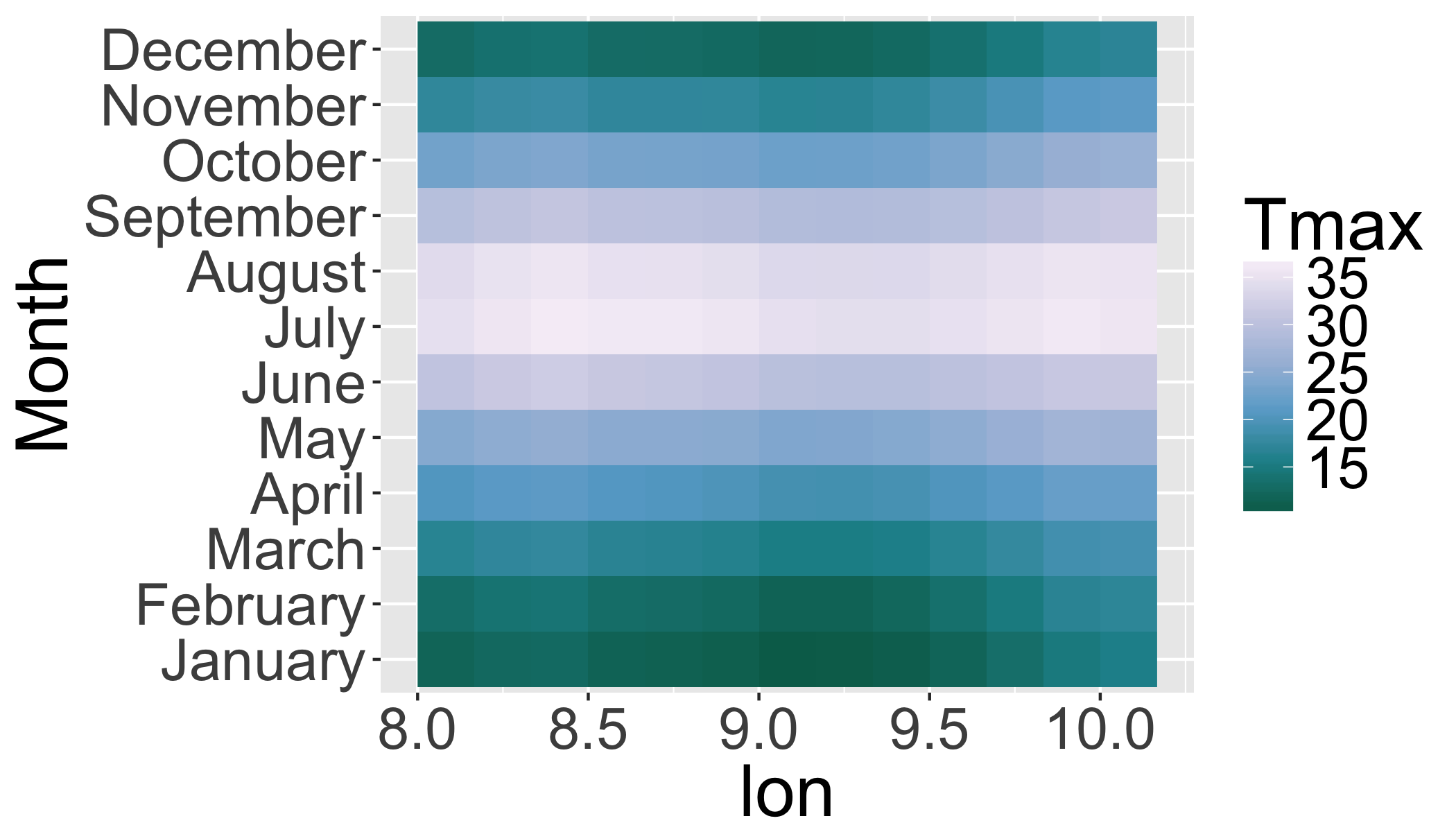
Or the same data in a levelplot:

ggplot(transl,
       aes(x=lon,y=monthname,
           fill=value))+
  ylab("Month")+
    scale_fill_distiller(
      palette="PuBuGn",
      name="Tmax")+
    geom_raster()

A quick introduction to spatial data analysis

1 Setup

2 Point data

2.1 Generate some random data

2.2 Convert to SpatialPoints

2.3 Create a SpatialPointsDataFrame

2.4 Promote a data frame with coordinates() to a SpatialPoints object

2.5 Subset data

2.5 Your turn

2.6 Examine topsoil quality in the Meuse river data set

2.6 Your turn

2.7 ggplot

3 Raster Package

3.1 getData()

3.2 GADM: Global Administrative Areas

3.2.1 Check out attribute table

3.2.1 Your turn

4 Raster Data

4.1 Raster introduction

4.2 Raster data storage

4.2 Your turn

4.3 Raster memory usage

4.4 Raster Plotting

4.4.1 ggplot and rasterVis

4.5 Spatial Projections

5 WorldClim

5.1 Overview of WorldClim

5.2 Bioclim variables

5.3 Download climate data

5.3.1 Gain and Offset

5.3.2 Plot with plot()

5.4 Faceting in ggplot

5.5 Subsetting and spatial cropping

5.6 Spatial aggregation

5.6 Your turn

5.7 Focal (“moving window”)

5.7 Your turn

5.8 Raster calculations

5.8.1 Apply algebraic functions

5.9 Extracting Raster Data

5.9.1 Point data

5.9.2 Extract data using a SpatialPoints object

5.9.3 Plot the global dataset with the random points

5.9.4 Summarize climate data at point locations

5.9.5 Lines

5.9.6 Plot Transect

5.9.6.1 Add other metadata and reshape

5.9.7 Zonal statistics

5.10 Example Workflow

5.11 Create a Transect (SpatialLinesDataFrame)

5.12 Plot the timeseries of climate data

5.13 Extract and clean up the transect data

5.14 Plot the transect data

2.2 Convert to `SpatialPoints`

2.3 Create a `SpatialPointsDataFrame`

2.4 Promote a data frame with `coordinates()` to a `SpatialPoints` object

3.1 `getData()`

5.3.2 Plot with `plot()`

5.9.2 Extract data using a `SpatialPoints` object