Introduction to Demography
Cory Merow
10/5/2017
This tutorial is a quick start guide stage structured demography.
Download the PDF of the presentation
The R Script associated with this page is available
Download this file and open it (or copy-paste into a new script) with RStudio so you can follow along.
1 Overview
We will conduct a simplified population viability analysis (PVA) for a rare herbacious perennial plant, Penstemon albomarginatus, for its only remaining California population. This (over)simplified PVA has two objectives:
Estimating the population growth rate - deterministic
- Sensitivity and elasticity analysis - which transitions/rate are most variable, sensitive to change
2 Introduction
What you need for a class/stage structured demographic model:
- a bunch of individuals (maybe in different populations)
- annual survival rates
- annual class or stage transition rates
- annual fecundity, ie. probability of contribution to the juvenile class in the next year
- these data for a lot of years (but we do what we can with less)
The crux for plants is that its challenging to 1) count all seeds produced annually and 2) know how many seeds result in a juvenile in any year. If you have a well behaved penguin that you can collar and track and you know it produces 2 live juveniles each season, your PVA might be a bit simpler.
Our field data had surivival for each year, mean plant diameter, and inflorescence count classes. From this I found the median inflorescence number for each class MEDIAN_INLF. I assigned each plant to CLASS based on its xDIAM_cm. I convinced myself that this had biological meaning by looking at the relationship between size class and survival. Whatever classes or stages you use, you should be confident that they are meaningful for your study species. OR use an integral projection model (IPM) instead. These allow you to use continuous variables like size or age rather than classes.
#  Load libraries
library(popbio)
library(plyr)
library(reshape)
##
## Attaching package: 'reshape'## The following objects are masked from 'package:plyr':
##
## rename, round_any# nice abbreviated dataset
andre <-read.csv("20_assets/Exercises/karadat.csv")
str(andre)## 'data.frame': 1221 obs. of 4 variables:
## $ PLANT_UNQ: Factor w/ 395 levels "1_703","1_704",..: 238 240 249 253 258 263 250 255 259 239 ...
## $ YEAR : int 1994 1994 1994 1994 1994 1994 1994 1994 1994 1994 ...
## $ CLASS : Factor w/ 6 levels "A1","A2","A3",..: 1 1 1 1 1 1 2 2 2 3 ...
## $ SEEDS : num 71.8 0 71.8 0 71.8 ...# look at the stages/classes
levels(andre$CLASS) # note that you need "dead" as a class for the first year that an individual is dead. After that it can be omitted.## [1] "A1" "A2" "A3" "A4" "dead" "J"There are 4 types of adults (A), juveniles (J), and dead individuals.
3 Estimating fecundity
The big challenge for plants = estimating seeds/indiv juveniles produced the next year based on a few fruit and seed counts and a lot of inflorescence class data. Ideally you would have seed counts for each plant, but in the absence of those nearly impossible data, I’m using a few seeds/fruit counts * fruits/infl counts from 2011 and 2012.
I’ll add some notes on how I made these estimates at the end of this script, but let’s start today with a dataset ready to go for popbio. See the SEEDS column:
str(andre)## 'data.frame': 1221 obs. of 4 variables:
## $ PLANT_UNQ: Factor w/ 395 levels "1_703","1_704",..: 238 240 249 253 258 263 250 255 259 239 ...
## $ YEAR : int 1994 1994 1994 1994 1994 1994 1994 1994 1994 1994 ...
## $ CLASS : Factor w/ 6 levels "A1","A2","A3",..: 1 1 1 1 1 1 2 2 2 3 ...
## $ SEEDS : num 71.8 0 71.8 0 71.8 ...# Here are the number in each class observed annually
(n_options<-ddply (andre, c("YEAR"), function (df) return(table(df$CLASS))))4 Pick a starting population vector
This is the # of individuals in each class/stage at the start of your model. You’ll use this to start simulations and see how the population changes. You should play around with this to see how it effects the outcome. My model is insensitive to realistic changes in this vector.
# picked starting population vector from 1995, the first year with 9 observed populations
n95<-c(81,31,17,13,11)
n=n95  # this must be called "n" for popbio

# notice that I only have J(uvenile) class individuals for a subset of the years.
5 Generate a transition matrix
This matrix links each individual to its fate in the next year/cycle/season. This is why you need each individual to be “dead” for a year, but no longer. If your raw data is like mine and only taken on live plants, “dead” might be something you have to add.
# make columns for year2, fate, and seeds2 for the whole census
trans<-subset(merge(andre, andre, by = "PLANT_UNQ", sort = FALSE), YEAR.x == YEAR.y - 1)

# rename rows and columns to improve clarity (I use the names used by popbio, which are similar to Morris and Doak)
#rownames(trans) <- 1:nrow(trans)
colnames(trans) <- c("plant",  "year", "stage", "seeds",  "year2", "fate", "seeds2")
head2(trans)
# add individual fertility estimates from the calculations above
seedlingtrans<-0.00305 # This is the rate at which a seed becomes a J individual (I estimated this elsewhere, see Appendix below)
# adding in the number of J individuals produced by each individual
trans$J<- trans$seeds * seedlingtrans # note that J is not an integer, which is totally fine, its a rate of J production
head2(trans)6 Generate Annual Matrices
The simple way for 3 easy years…
#################     NAME STAGES   ###########################
stages <- c("J", "A1", "A2", "A3", "A4")
# you must have a vector of named stages in this way for your own classes

#################   SET ITERATIONS  ############################
it<-100        # set the number of time steps for a deterministic model

# Make a demographic projection matrix for each year like so:

#     1994
trans94 <-subset(trans, year == 1994, c(plant, stage, fate, J))
(proj94<-projection.matrix(trans94, stage, fate, J, sort = stages))  #this gives you a projection matrix for 1994
##
## J A1 A2 A3 A4
## J 0.07692308 0.14589167 0.78781500 0.78781500 4.35486625
## A1 0.53846154 0.33333333 0.33333333 0.00000000 0.00000000
## A2 0.07692308 0.33333333 0.00000000 0.00000000 0.00000000
## A3 0.00000000 0.16666667 0.33333333 0.50000000 0.00000000
## A4 0.00000000 0.00000000 0.33333333 0.50000000 1.00000000# you can do a simple deterministic projection of the matrix for just this year
(p94<-pop.projection(proj94, n, it))## $lambda
## [1] 1.495539
##
## $stable.stage
##          J         A1         A2         A3         A4
## 0.48307335 0.24671015 0.07983487 0.06803345 0.12234818
##
## $stage.vectors
## 0 1 2 3 4 5 6 7
## J 81 82.29139 142.62014 223.46217 338.77859 502.17175 745.3968 1112.4949
## A1 31 59.61538 69.70391 108.76406 167.98228 256.22803 383.1608 570.4338
## A2 17 16.56410 26.20190 34.20542 53.44409 82.05398 124.0379 185.0585
## A3 13 17.33333 24.12393 32.41325 45.73578 68.67963 104.3958 157.4040
## A4 11 23.16667 37.35470 58.15063 85.75907 126.44165 188.1328 281.6767
## 8 9 10 11 12 13 14
## J 1665.2594 2492.9837 3729.5854 5577.2842 8339.954 12472.093 18652.619
## A1 850.8665 1272.2073 1903.6846 2848.0789 4259.664 6370.093 9526.248
## A2 275.7211 411.7190 615.8371 921.4527 1378.381 2061.423 3082.756
## A3 235.4605 351.4484 524.9984 785.0590 1174.360 1756.585 2627.115
## A4 422.0649 631.7021 944.6660 1412.4442 2112.125 3158.765 4724.198
## 15 16 17 18 19 20 21
## J 27896.192 41720.174 62394.16 93312.73 139552.72 208706.59 312129.02
## A1 14246.719 21306.677 31865.19 47655.74 71270.99 106588.49 159407.24
## A2 4610.233 6894.767 10311.47 15421.28 23063.15 34491.82 51583.85
## A3 3928.851 5875.623 8787.18 13141.61 19653.86 29393.14 43958.59
## A4 7065.341 10566.511 15802.58 23633.32 35344.56 52859.20 79053.05
## 22 23 24 25 26 27 28
## J 466801.33 698119.83 1044065.7 1561441.5 2335197.3 3492379.7 5222991.7
## A1 238399.83 356536.40 533214.3 797443.0 1192607.4 1783591.5 2667431.5
## A2 77145.67 115374.41 172547.0 258050.8 385925.2 577166.4 863175.1
## A3 65741.79 98319.42 147040.6 219905.0 328876.6 491848.0 735578.0
## A4 118226.96 176813.08 264430.9 395466.9 591436.3 884516.4 1322829.1
## 29 30 31 32 33 34 35 36
## J 7811190 11681943 17470807 26128282 39075876 58439515 87398601 130708056
## A1 3989249 5966079 8922507 13343961 19956421 29845615 44635295 66753845
## A2 1290912 1930610 2887304 4318077 6457855 9657977 14443886 21601401
## A3 1100086 1645222 2460494 3679766 5503236 8230306 12308748 18408218
## A4 1978343 2958690 4424838 6617520 9896762 14800999 22135477 33104480
## 37 38 39 40 41 42 43
## J 195479056 292346643 437215941 653873694 977893912 1462478936 2187194963
## A1 99833010 149304206 223290332 333939503 499419705 746901877 1117021232
## A2 32305748 48314520 72256272 108062106 161611144 241695844 361465672
## A3 27530217 41172526 61575137 92088048 137721310 205967654 308032754
## A4 49509056 74042747 110733850 165606843 247671569 370402605 553951713
## 44 45 46 47 48 49
## J 3271036379 4891963989 7316125196 10941553944 16363525705 24472298441
## A1 1670549332 2498372451 3736414593 5587955472 8357007924 12498235141
## A2 540586177 808467960 1209095739 1808250392 2704309820 4044402055
## A3 460675140 688957851 1030363654 1540949506 2304550796 3446546658
## A4 828456648 1238989610 1852957856 2771171596 4144396479 6198108484
## 50 51 52 53 54
## J 36599288060 54735679599 81859368856 122423916512 183089798317
## A1 18691603867 27954031203 41806356804 62523056391 93505698158
## A2 6048562876 9045864473 13528447293 20232326795 30258243144
## A3 5154446538 7708678205 11528632461 17241524795 25785380728
## A4 9269515831 13862926725 20732553985 31006352647 46371223976
## 55 56 57 58 59
## J 273818018594 409505652393 612431863336 915916019808 1.369789e+12
## A1 139841461579 209138424308 312774766710 467767006539 6.995640e+11
## A2 45252396693 67676745034 101213242902 151368398904 2.263774e+11
## A3 38563054438 57672569713 86251603919 128992677379 1.929136e+11
## A4 69349995388 103715654838 155110854706 231974404300 3.469269e+11
## 60 61 62 63 64
## J 2.048573e+12 3.063722e+12 4.581916e+12 6.852437e+12 1.024809e+13
## A1 1.046226e+12 1.564672e+12 2.340028e+12 3.499605e+12 5.233797e+12
## A2 3.385564e+11 5.063244e+11 7.572281e+11 1.132465e+12 1.693645e+12
## A3 2.885100e+11 4.314780e+11 6.452924e+11 9.650603e+11 1.443286e+12
## A4 5.188428e+11 7.759499e+11 1.160464e+12 1.735519e+12 2.595538e+12
## 65 66 67 68 69
## J 1.532642e+13 2.292127e+13 3.427966e+13 5.126659e+13 7.667121e+13
## A1 7.827350e+12 1.170611e+13 1.750695e+13 2.618233e+13 3.915671e+13
## A2 2.532913e+12 3.788072e+12 5.665211e+12 8.472547e+12 1.267103e+13
## A3 2.158491e+12 3.228108e+12 4.827763e+12 7.220110e+12 1.079796e+13
## A4 3.881729e+12 5.805279e+12 8.682024e+12 1.298431e+13 1.941855e+13
## 70 71 72 73 74
## J 1.146648e+14 1.714858e+14 2.564637e+14 3.835516e+14 5.736166e+14
## A1 5.856041e+13 8.757940e+13 1.309785e+14 1.958834e+14 2.929514e+14
## A2 1.895002e+13 2.834051e+13 4.238435e+13 6.338746e+13 9.479845e+13
## A3 1.614877e+13 2.415113e+13 3.611897e+13 5.401734e+13 8.078507e+13
## A4 2.904120e+13 4.343226e+13 6.495467e+13 9.714227e+13 1.452801e+14
## 75 76 77 78 79
## J 8.578662e+14 1.282973e+15 1.918736e+15 2.869546e+15 4.291519e+15
## A1 4.381204e+14 6.552264e+14 9.799169e+14 1.465504e+15 2.191720e+15
## A2 1.417748e+14 2.120299e+14 3.170990e+14 4.742341e+14 7.092358e+14
## A3 1.208173e+14 1.806870e+14 2.702245e+14 4.041314e+14 6.043945e+14
## A4 2.172721e+14 3.249390e+14 4.859591e+14 7.267710e+14 1.086915e+15
## 80 81 82 83 84
## J 6.418137e+15 9.598577e+15 1.435505e+16 2.146854e+16 3.210705e+16
## A1 3.277803e+15 4.902084e+15 7.331260e+15 1.096419e+16 1.639738e+16
## A2 1.060690e+15 1.586304e+15 2.372380e+15 3.547988e+15 5.306156e+15
## A3 9.038958e+14 1.351812e+15 2.021688e+15 3.023514e+15 4.521785e+15
## A4 1.625524e+15 2.431035e+15 3.635709e+15 5.437346e+15 8.131766e+15
## 85 86 87 88 89
## J 4.801737e+16 7.181187e+16 1.073975e+17 1.606172e+17 2.402093e+17
## A1 2.452293e+16 3.667500e+16 5.484891e+16 8.202871e+16 1.226772e+17
## A2 7.935566e+15 1.186795e+16 1.774899e+16 2.654432e+16 3.969807e+16
## A3 6.762507e+15 1.011360e+16 1.512528e+16 2.262046e+16 3.382979e+16
## A4 1.216138e+16 1.818782e+16 2.720060e+16 4.067957e+16 6.083791e+16
## 90 91 92 93 94
## J 3.592425e+17 5.372614e+17 8.034956e+17 1.201659e+18 1.797129e+18
## A1 1.834686e+17 2.743845e+17 4.103528e+17 6.136988e+17 9.178108e+17
## A2 5.937003e+16 8.879023e+16 1.327893e+17 1.985916e+17 2.970016e+17
## A3 5.059378e+16 7.566499e+16 1.131600e+17 1.692352e+17 2.530980e+17
## A4 9.098549e+16 1.360724e+17 2.035016e+17 3.043447e+17 4.551595e+17
## 95 96 97 98 99
## J 2.687677e+18 4.019527e+18 6.011362e+18 8.990229e+18 1.344524e+19
## A1 1.372622e+18 2.052811e+18 3.070060e+18 4.591395e+18 6.866613e+18
## A2 4.441776e+17 6.642852e+17 9.934647e+17 1.485766e+18 2.222021e+18
## A3 3.785180e+17 5.660886e+17 8.466078e+17 1.266135e+18 1.893555e+18
## A4 6.807091e+17 1.018027e+18 1.522500e+18 2.276959e+18 3.405282e+18
##
## $pop.sizes
## [1] 1.530000e+02 1.989709e+02 3.000046e+02 4.569955e+02 6.916998e+02
## [6] 1.035575e+03 1.545124e+03 2.307068e+03 3.449372e+03 5.160061e+03
## [11] 7.718772e+03 1.154432e+04 1.726448e+04 2.581896e+04 3.861294e+04
## [16] 5.774734e+04 8.636375e+04 1.291606e+05 1.931647e+05 2.888853e+05
## [21] 4.320392e+05 6.461317e+05 9.663156e+05 1.445163e+06 2.161298e+06
## [26] 3.232307e+06 4.834043e+06 7.229502e+06 1.081201e+07 1.616978e+07
## [31] 2.418255e+07 3.616595e+07 5.408761e+07 8.089015e+07 1.209744e+08
## [36] 1.809220e+08 2.705760e+08 4.046571e+08 6.051806e+08 9.050715e+08
## [41] 1.353570e+09 2.024318e+09 3.027447e+09 4.527666e+09 6.771304e+09
## [46] 1.012675e+10 1.514496e+10 2.264988e+10 3.387379e+10 5.065959e+10
## [51] 7.576342e+10 1.133072e+11 1.694554e+11 2.534272e+11 3.790103e+11
## [56] 5.668249e+11 8.477090e+11 1.267782e+12 1.896019e+12 2.835570e+12
## [61] 4.240708e+12 6.342146e+12 9.484929e+12 1.418509e+13 2.121436e+13
## [66] 3.172691e+13 4.744884e+13 7.096161e+13 1.061259e+14 1.587155e+14
## [71] 2.373652e+14 3.549891e+14 5.309002e+14 7.939821e+14 1.187432e+15
## [76] 1.775851e+15 2.655855e+15 3.971936e+15 5.940187e+15 8.883784e+15
## [81] 1.328605e+16 1.986981e+16 2.971609e+16 4.444158e+16 6.646414e+16
## [86] 9.939974e+16 1.486562e+17 2.223213e+17 3.324902e+17 4.972523e+17
## [91] 7.436604e+17 1.112173e+18 1.663299e+18 2.487530e+18 3.720199e+18
## [96] 5.563704e+18 8.320739e+18 1.244399e+19 1.861048e+19 2.783271e+19
##
## $pop.changes
## [1] 1.300463 1.507781 1.523295 1.513581 1.497145 1.492045 1.493128
## [8] 1.495133 1.495942 1.495868 1.495616 1.495496 1.495496 1.495526
## [15] 1.495544 1.495545 1.495542 1.495539 1.495539 1.495539 1.495539
## [22] 1.495540 1.495540 1.495539 1.495539 1.495539 1.495539 1.495539
## [29] 1.495539 1.495539 1.495539 1.495539 1.495539 1.495539 1.495539
## [36] 1.495539 1.495539 1.495539 1.495539 1.495539 1.495539 1.495539
## [43] 1.495539 1.495539 1.495539 1.495539 1.495539 1.495539 1.495539
## [50] 1.495539 1.495539 1.495539 1.495539 1.495539 1.495539 1.495539
## [57] 1.495539 1.495539 1.495539 1.495539 1.495539 1.495539 1.495539
## [64] 1.495539 1.495539 1.495539 1.495539 1.495539 1.495539 1.495539
## [71] 1.495539 1.495539 1.495539 1.495539 1.495539 1.495539 1.495539
## [78] 1.495539 1.495539 1.495539 1.495539 1.495539 1.495539 1.495539
## [85] 1.495539 1.495539 1.495539 1.495539 1.495539 1.495539 1.495539
## [92] 1.495539 1.495539 1.495539 1.495539 1.495539 1.495539 1.495539
## [99] 1.495539(l94<-p94$lambda) # wow! if we looked only at 1994 based on these estimates the population would be booming!## [1] 1.495539# stable.stage shows the proportion of the population in each stage class at the mythical equilibrium, 48% of plants are juveniles in 100 years
p94$stable.stage## J A1 A2 A3 A4
## 0.48307335 0.24671015 0.07983487 0.06803345 0.12234818# Now make some matrices for other years
# 1995
trans95 <-subset(trans, year == 1995, c(plant, stage, fate, J))
(proj95<-projection.matrix(trans95, stage, fate, J, sort = stages))##
## J A1 A2 A3 A4
## J 0.20000000 0.26260500 1.02982353 3.52160038 6.21498500
## A1 0.21250000 0.74193548 0.47058824 0.07692308 0.00000000
## A2 0.00000000 0.12903226 0.47058824 0.15384615 0.09090909
## A3 0.00000000 0.00000000 0.00000000 0.76923077 0.36363636
## A4 0.00000000 0.00000000 0.00000000 0.00000000 0.54545455# 2011
trans11 <-subset(trans, year == 2011, c(plant, stage, fate, J))
(proj11<-projection.matrix(trans11, stage, fate, J, sort = stages))##
## J A1 A2 A3 A4
## J 0.15733432 0.98329042 4.57099692 8.06477464 7.92191750
## A1 0.00000000 0.05555556 0.30769231 0.14285714 0.00000000
## A2 0.00000000 0.00000000 0.00000000 0.00000000 0.50000000
## A3 0.00000000 0.00000000 0.00000000 0.00000000 0.00000000
## A4 0.00000000 0.00000000 0.00000000 0.14285714 0.00000000p95<-pop.projection(proj95, n, it)
(l95<-p95$lambda) # lambda is much lower in 1995## [1] 0.9954251(p11<-pop.projection(proj11, n, pi))## $lambda
## [1] 0.3064825
##
## $stable.stage
## J A1 A2 A3 A4
## 0.969161385 0.021631924 0.009206691 0.000000000 0.000000000
##
## $stage.vectors
## 0 1 2
## J 81 312.916193 97.7479930
## A1 31 8.810134 2.1817596
## A2 17 5.500000 0.9285714
## A3 13 0.000000 0.0000000
## A4 11 1.857143 0.0000000
##
## $pop.sizes
## [1] 153.0000 329.0835 100.8583
##
## $pop.changes
## [1] 2.1508724 0.3064825(l11<-p11$lambda) # and based on 2011 alone extinction is eminent. The gist here is we need lots of years of data to make any decent estimation of what the population is really likely to do (ie more than the three here)## [1] 0.30648257 Deterministic Population Viability Analysis
thesearethemeanprojmats<-list(proj94, proj95, proj11)  # make a list of the three matrices
(meanxprojmat <-mean(thesearethemeanprojmats))   # make a mean of the three projection matrices for deterministic analysis
##
## J A1 A2 A3 A4
## J 0.14475247 0.46392903 2.1295452 4.12473001 6.1639229
## A1 0.25032051 0.37694146 0.3705380 0.07326007 0.0000000
## A2 0.02564103 0.15412186 0.1568627 0.05128205 0.1969697
## A3 0.00000000 0.05555556 0.1111111 0.42307692 0.1212121
## A4 0.00000000 0.00000000 0.1111111 0.21428571 0.5151515n # n is our starting population vector, ie the # of individuals in each class at the start of the projection## [1] 81 31 17 13 11(pprojme <- pop.projection(meanxprojmat, n)) # do the deterministic projection, lambda is the dominant left eigenvalue## $lambda
## [1] 1.088618
##
## $stable.stage
## J A1 A2 A3 A4
## 0.61435772 0.25469431 0.06677005 0.03730232 0.02687559
##
## $stage.vectors
## 0 1 2 3 4 5 6
## J 81 183.73366 177.920994 182.074264 196.519009 214.113465 233.25714
## A1 31 39.21267 66.116232 75.791265 82.085465 88.980306 96.74873
## A2 17 12.35470 15.265171 19.380118 21.551041 23.374214 25.37951
## A3 13 10.44444 9.223517 10.354925 11.748187 12.972066 14.16333
## A4 11 10.34127 8.938161 8.277105 8.636222 9.360992 10.19919
## 7 8 9 10 11 12 13
## J 253.98286 276.50191 301.00620 327.68051 356.71869 388.33030 422.74331
## A1 105.29933 114.62868 124.78748 135.84629 147.88483 160.99011 175.25672
## A2 27.60840 30.05113 32.71391 35.61308 38.76912 42.20478 45.94488
## A3 15.42332 16.78937 18.27658 19.89601 21.65910 23.57848 25.66796
## A4 11.10907 12.09545 13.16773 14.33466 15.60496 16.98784 18.49326
## 14 15 16 17 18 19
## J 460.20594 500.98844 545.38499 593.71588 646.32974 703.60614
## A1 190.78760 207.69480 226.10029 246.13682 267.94896 291.69404
## A2 50.01642 54.44877 59.27391 64.52664 70.24486 76.46981
## A3 27.94260 30.41881 33.11447 36.04900 39.24359 42.72127
## A4 20.13209 21.91616 23.85832 25.97260 28.27424 30.77984
##
## $pop.sizes
## [1] 153.0000 256.0867 277.4641 295.8777 320.5399 348.8010 379.7479
## [8] 413.4230 450.0665 489.9519 533.3706 580.6367 632.0915 688.1061
## [15] 749.0847 815.4670 887.7320 966.4009 1052.0414 1145.2711
##
## $pop.changes
## [1] 1.673770 1.083477 1.066364 1.083353 1.088167 1.088724 1.088677
## [8] 1.088635 1.088621 1.088618 1.088618 1.088618 1.088618 1.088618
## [15] 1.088618 1.088618 1.088618 1.088618 1.088618(DetLamb<-pprojme$lambda)## [1] 1.088618# calculate fertility and survival sums as useful summaries of the projection matrix
(projsums <- colSums(meanxprojmat))## J A1 A2 A3 A4
## 0.420714 1.050548 2.879168 4.886635 6.997256(fert_row <- meanxprojmat[1,]) # expected number of juveniles from an individual in each age class## J A1 A2 A3 A4
## 0.1447525 0.4639290 2.1295452 4.1247300 6.1639229(surv_row <- projsums-fert_row) # survival probability of an individual in each age class## J A1 A2 A3 A4
## 0.2759615 0.5866189 0.7496229 0.7619048 0.83333338 Appendix: Sensitivity and Elasticity
SENSITIVITY is a measure of the amount of change in λ give a small change in a matrix element.
ELASTICITY is a measure of `proportional’ effect, i.e., the effect that a change in a given matrix element has as a proportional to the change in that element
meanxprojmat # for an overall look at sensitivity and elasticity use the mean projection matrix##
## J A1 A2 A3 A4
## J 0.14475247 0.46392903 2.1295452 4.12473001 6.1639229
## A1 0.25032051 0.37694146 0.3705380 0.07326007 0.0000000
## A2 0.02564103 0.15412186 0.1568627 0.05128205 0.1969697
## A3 0.00000000 0.05555556 0.1111111 0.42307692 0.1212121
## A4 0.00000000 0.00000000 0.1111111 0.21428571 0.5151515# you could do separate analyses by year or type of year too to examine how sensitivity and elasticity vary among years
(eigout <- eigen.analysis(meanxprojmat)) # do the associated sensitivity analysis## $lambda1
## [1] 1.088618
##
## $stable.stage
## J A1 A2 A3 A4
## 0.61435772 0.25469431 0.06677005 0.03730232 0.02687559
##
## $sensitivities
##
## J A1 A2 A3 A4
## J 0.2255489 0.09350582 0.02451326 0.01369479 0.009866825
## A1 0.6929862 0.28729131 0.07531560 0.04207645 0.000000000
## A2 1.5373471 0.63733809 0.16708303 0.09334402 0.067252539
## A3 0.0000000 1.13131204 0.29658206 0.16569105 0.119377153
## A4 0.0000000 0.00000000 0.38355775 0.21428163 0.154385715
##
## $elasticities
##
##               J         A1         A2          A3         A4
##   J  0.02999102 0.03984875 0.04795263 0.051889003 0.05586749
##   A1 0.15934760 0.09947660 0.02563552 0.002831594 0.00000000
##   A2 0.03621028 0.09023160 0.02407557 0.004397202 0.01216838
##   A3 0.00000000 0.05773437 0.03027101 0.064393631 0.01329204
##   A4 0.00000000 0.00000000 0.03914829 0.042179622 0.07305780
##
## $repro.value
## J A1 A2 A3 A4
## 1.000000 3.072443 6.816026 12.098841 15.646949
##
## $damping.ratio
## [1] 4.215209colSums(eigout$elasticities) # this gives the cumulative elasticity of each stage/class. Note that these sum to 1, so you can determine which class has the biggest effect on lambda, if perturbed## J A1 A2 A3 A4
## 0.2255489 0.2872913 0.1670830 0.1656911 0.1543857Note that the elasticities are just the sensitivities multiplied by the projection matrix elements. Hence, elasticity up (down) weights the sensitivity for transitions that are(n’t) likely. The sum below just normalizes the elasticities to ensure they sum to 1.
eigout$elasticities##
## J A1 A2 A3 A4
## J 0.02999102 0.03984875 0.04795263 0.051889003 0.05586749
## A1 0.15934760 0.09947660 0.02563552 0.002831594 0.00000000
## A2 0.03621028 0.09023160 0.02407557 0.004397202 0.01216838
## A3 0.00000000 0.05773437 0.03027101 0.064393631 0.01329204
## A4 0.00000000 0.00000000 0.03914829 0.042179622 0.07305780eigout$sensitivities*meanxprojmat/sum(eigout$sensitivities*meanxprojmat)##
## J A1 A2 A3 A4
## J 0.02999102 0.03984875 0.04795263 0.051889003 0.05586749
## A1 0.15934760 0.09947660 0.02563552 0.002831594 0.00000000
## A2 0.03621028 0.09023160 0.02407557 0.004397202 0.01216838
## A3 0.00000000 0.05773437 0.03027101 0.064393631 0.01329204
## A4 0.00000000 0.00000000 0.03914829 0.042179622 0.07305780Here, we calculate the summed elasticity for each class to get a sense of which life stages contribute most to population growth. You could also pick the vital rates (matrix elements) that are most meaningful in your own analysis
(fert_row_e <- eigout$elasticities[1,])## J A1 A2 A3 A4
## 0.02999102 0.03984875 0.04795263 0.05188900 0.05586749(surv_row_e <-apply(eigout$elasticities[2:5,],2,sum))## J A1 A2 A3 A4
## 0.19555788 0.24744256 0.11913039 0.11380205 0.09851822par(mfrow=c(1,2))
barplot(surv_row_e,xlab="Stage class",main="Elasticity for Growth and Survival")
barplot(fert_row_e, xlab="Stage class",main="Elasticity for Fertility")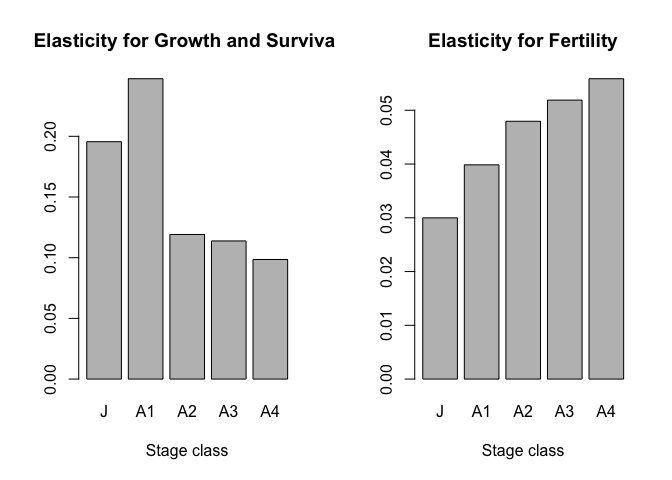
Not surprisingly, small adult growth and survival contributes most to lambda while large adult reproduction is the most important component of fertility.
9 Appendix: Generating a fecundity estimate
I’m including this for plant folks who might like to see how I made fecundity estimates from real data. I also have developed a script to simulate juvenile numbers and transition rates for the years in my dataset that are missing these data, and bootstraps of the whole model.
#  Load up the raw-ish data

andre <-read.csv ("20_assets/Exercises/D__composite9_13_2012.csv")
str(andre)
## 'data.frame': 1693 obs. of 15 variables:
## $ PLANT_UNQ : Factor w/ 619 levels "1_701","1_702",..: 462 464 473 477 482 487 474 479 483 463 ...
## $ YEAR : int 1994 1994 1994 1994 1994 1994 1994 1994 1994 1994 ...
## $ CLASS : Factor w/ 6 levels "A1","A2","A3",..: 1 1 1 1 1 1 2 2 2 3 ...
## $ OBS_ID : int 1 3 20 24 11 16 21 26 12 2 ...
## $ COHORT : Factor w/ 18 levels "1","2","3","4",..: 10 10 11 11 11 11 11 11 11 10 ...
## $ PLANT.NUM : Factor w/ 460 levels "1","10","11",..: 1 23 5 9 41 168 6 11 42 12 ...
## $ xDIAM_cm : num 12 11 17 12 18 12 23 22 29 32 ...
## $ SEEDS_DC : num 26.7 26.7 26.7 26.7 26.7 ...
## $ MEDIAN_INFL : int 5 0 5 0 5 5 18 18 18 18 ...
## $ INFL_CLASS : int 1 0 1 0 1 1 2 2 2 2 ...
## $ MAX_INFL : int 111 0 111 0 111 111 123 123 123 123 ...
## $ OBS_INLF : int NA NA NA NA NA NA NA NA NA NA ...
## $ SEEDS_YR_INF: num NA NA NA NA NA NA NA NA NA NA ...
## $ CAGED : Factor w/ 2 levels "N","Y": 1 1 1 1 1 1 1 1 1 1 ...
## $ WATERED : Factor w/ 2 levels "N","Y": 1 1 1 1 1 1 1 1 1 1 ...# BEST ESTIMATE OF SEED PRODUCTION: average of seeds/fruit, weighed average of fruits/infl where 0.14 is 1/8 drought years
andre$SEEDS<-andre$MEDIAN_INFL * 14.35 # = 14.35 seeds/infl
# The big crux Part 2: How many seeds makes a J plant the next year?
# ie what is the transition rate or fecundity rate?
# observed juveniles in each year (sadly not all years have the same # of cohorts, so I adjust for that below)
seedling_yr<-ddply (andre, c("YEAR"), function (df)
return(c(sdlgs=sum(df$CLASS == "J")))) # shows the OBSERVED # of J plants each year,
# and some of these are not observation years and are omitted below
seedling_yr#seedlings for 9 cohorts based on census from each year
sdl94=seedling_yr$sdlgs[(seedling_yr$YEAR=="1994")]*9/2 # this year had only 2 cohorts
sdl95=seedling_yr$sdlgs[(seedling_yr$YEAR=="1995")]
sdl11=seedling_yr$sdlgs[(seedling_yr$YEAR=="2011")]
sdl12=0 # in 2012 observed seedlings were 0
seedling_pick=c(sdl94,sdl95,sdl11, sdl12)
seedling_pick## [1] 58.5 81.0 362.0 0.0# estimate seedlings as the mean of the 4 OBSERVED years:
# in the other years seedlings where not surveyed for
(seedlings=mean(seedling_pick)) # = 125.375 seedlings/year on average## [1] 125.375# what's the annual total seed production rate?
# add up all the seeds estimated to be produced in each year
seed_yr<-ddply (andre, c("YEAR"), function (df)
return(c(sumseeds=sum(df$SEEDS))))
seed_yr# adjust so that 1994 has an estimate of all cohorts based on the observed 2 cohorts
seed_yr$sumseeds[(seedling_yr$YEAR=="1994")]<-(seed_yr$sumseeds[(seedling_yr$YEAR=="1994")]*9/2)
# get mean seeds/year
avg_seeds_p_yr<-mean(seed_yr$sumseeds)
# for each of the 4 years in which seedlings were observed, calculate an estimate of the transition rate from seed --> J
str(sdl.trans94<-sdl94/avg_seeds_p_yr)## num 0.00179str(sdl.trans95<-sdl95/avg_seeds_p_yr)## num 0.00247str(sdl.trans11<-sdl11/avg_seeds_p_yr)## num 0.011sdl.trans12<-0 # no seedlings observed this year
# looks at the options for transition rate
str(seedlingtrans_pick<-c(sdl.trans94,sdl.trans95,sdl.trans11,sdl.trans12))## num [1:4] 0.00179 0.00247 0.01105 0# pick the mean for this analysis
(seedlingtrans<-mean(seedlingtrans_pick)) # mean seedling transition rate 0.00305## [1] 0.003825986### Now remove watered and caged plants from main dataset, these have different survival and transition rates.
# I included them thus far because we needed to get seed production estimates for them. Since they might have contributed
# to the observed juveniles
andre<-andre[(andre$CAGED =="N"),]
andre<-andre[(andre$WATERED =="N"),]
head2(andre)# reduce datafile to include only PLANT_UNQ, YEAR, CLASS and SEEDS
str(andre)## 'data.frame': 1221 obs. of 16 variables:
## $ PLANT_UNQ : Factor w/ 619 levels "1_701","1_702",..: 462 464 473 477 482 487 474 479 483 463 ...
## $ YEAR : int 1994 1994 1994 1994 1994 1994 1994 1994 1994 1994 ...
## $ CLASS : Factor w/ 6 levels "A1","A2","A3",..: 1 1 1 1 1 1 2 2 2 3 ...
## $ OBS_ID : int 1 3 20 24 11 16 21 26 12 2 ...
## $ COHORT : Factor w/ 18 levels "1","2","3","4",..: 10 10 11 11 11 11 11 11 11 10 ...
## $ PLANT.NUM : Factor w/ 460 levels "1","10","11",..: 1 23 5 9 41 168 6 11 42 12 ...
## $ xDIAM_cm : num 12 11 17 12 18 12 23 22 29 32 ...
## $ SEEDS_DC : num 26.7 26.7 26.7 26.7 26.7 ...
## $ MEDIAN_INFL : int 5 0 5 0 5 5 18 18 18 18 ...
## $ INFL_CLASS : int 1 0 1 0 1 1 2 2 2 2 ...
## $ MAX_INFL : int 111 0 111 0 111 111 123 123 123 123 ...
## $ OBS_INLF : int NA NA NA NA NA NA NA NA NA NA ...
## $ SEEDS_YR_INF: num NA NA NA NA NA NA NA NA NA NA ...
## $ CAGED : Factor w/ 2 levels "N","Y": 1 1 1 1 1 1 1 1 1 1 ...
## $ WATERED : Factor w/ 2 levels "N","Y": 1 1 1 1 1 1 1 1 1 1 ...
## $ SEEDS : num 71.8 0 71.8 0 71.8 ...str(andre<-andre[,c(1:3,16)])## 'data.frame': 1221 obs. of 4 variables:
## $ PLANT_UNQ: Factor w/ 619 levels "1_701","1_702",..: 462 464 473 477 482 487 474 479 483 463 ...
## $ YEAR : int 1994 1994 1994 1994 1994 1994 1994 1994 1994 1994 ...
## $ CLASS : Factor w/ 6 levels "A1","A2","A3",..: 1 1 1 1 1 1 2 2 2 3 ...
## $ SEEDS : num 71.8 0 71.8 0 71.8 ...# Go back to step 2.10 Colophon
- Exercises are based on materials developed by Kara Moore